Week 13: Course Wrapup

DSAN 5000: Data Science and Analytics

Open slides in new window →

Student Presentations

source("../_globals.r")

cb_palette = ["#E69F00", "#56B4E9", "#009E73", "#F0E442", "#0072B2", "#D55E00", "#CC79A7"]

from IPython.display import Markdown
def disp(df, floatfmt='g', include_index=True):
  return Markdown(
    df.to_markdown(
      floatfmt=floatfmt,
      index=include_index
    )
  )

def summary_to_df(summary_obj, corner_col = ''):
    reg_df = pd.DataFrame(summary_obj.tables[1].data)
    reg_df.columns = reg_df.iloc[0]
    reg_df = reg_df.iloc[1:].copy()
    # Save index col
    index_col = reg_df['']
    # Drop for now, so it's all numeric
    reg_df.drop(columns=[''], inplace=True)
    reg_df = reg_df.apply(pd.to_numeric)
    my_round = lambda x: round(x, 2)
    reg_df = reg_df.apply(my_round)
    numeric_cols = reg_df.columns
    # Add index col back in
    reg_df.insert(loc=0, column=corner_col, value=index_col)
    # Sigh. Have to escape | characters?
    reg_df.columns = [c.replace("|","\|") for c in reg_df.columns]
    return reg_df

$$$$

Course Recap

(Why Do A Course Recap?)

Data = Ground Truth + Noise

• Depressing but true origin of statistics (as opposed to probability): the Plague 😷

Ground Truth: The Great Plague (Lord Have Mercy on London, Unknown Artist, circa 1665, via Wikimedia Commons)

Noisy Data (Recorded amidst chaos): London Bill of Mortality, 1665 (Public Domain, Wellcome Collection)

Your Toolbox

Basics

• GitHub
• File Formats
• Web Scraping

Nuts and Bolts

• Data-Generating Processes (DGPs)
• Distance Metrics
• Entropy
• Gaussian / Normal Distributions
• Clustering
• Dimensionality Reduction

Drills and Saws

• Decision Trees

GitHub (W03)

Data Structures: Simple $\to$ Complex (W04)

id	name	email
0	K. Desbrow	kd9@dailymail.com
1	D. Minall	dminall1@wired.com
2	C. Knight	ck2@microsoft.com
3	M. McCaffrey	mccaf4@nhs.uk

Figure 1: Record Data

year	month	points
2023	Jan	65
2023	Feb
2023	Mar	42
2023	Apr	11

Figure 2: Time-Series Data

id	date	rating	num_rides
0	2023-01	0.75	45
0	2023-02	0.89	63
0	2023-03	0.97	7
1	2023-06	0.07	10

Figure 3: Panel Data

id	Source	Target	Weight
1	IGF2	IGF1R	1
2	IGF1R	TP53	2
3	TP53	EGFR	0.5

Figure 4: Network Data

Web Scraping (W04)

		How is data loaded?	Solution	Example
😊	Easy	Data in HTML source	“View Source”
😐	Medium	Data loaded dynamically via API	“View Source”, find API call, scrape programmatically
😳	Hard	Data loaded dynamically [internally] via web framework	Use Selenium

EDA: Why We Can’t Just Skip It (W06)

• Iterative process: Ask questions of the data, find answers, generate more questions
• You’re probably already used to Mean and Variance: Fancier EDA/robustness methods build upon these two!
• Why do we need to visualize? Can’t we just use mean, $R^2$?
• …Enter Anscombe’s Quartet

import pandas as pd
import numpy as np
import matplotlib.pyplot as plt
import seaborn as sns
sns.set_theme(style="ticks")
# https://towardsdatascience.com/how-to-use-your-own-color-palettes-with-seaborn-a45bf5175146
sns.set_palette(sns.color_palette(cb_palette))

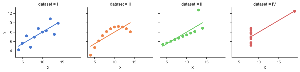
# Load the example dataset for Anscombe's quartet
anscombe_df = sns.load_dataset("anscombe")
#print(anscombe_df)

# Show the results of a linear regression within each dataset
anscombe_plot = sns.lmplot(
    data=anscombe_df, x="x", y="y", col="dataset", hue="dataset",
    col_wrap=4, palette="muted", ci=None,
    scatter_kws={"s": 50, "alpha": 1},
    height=3
);
anscombe_plot;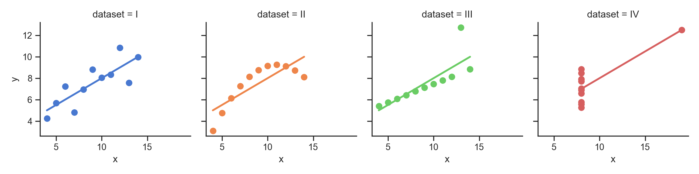

The Scariest Dataset of All Time

Summary statistics

# Compute dataset means
my_round = lambda x: round(x,2)
data_means = anscombe_df.groupby('dataset').agg(
  x_mean = ('x', np.mean),
  y_mean = ('y', np.mean)
).apply(my_round)

disp(data_means, floatfmt='.2f')

<string>:1: FutureWarning: The provided callable <function mean at 0x1338d9940> is currently using SeriesGroupBy.mean. In a future version of pandas, the provided callable will be used directly. To keep current behavior pass the string "mean" instead.
<string>:1: FutureWarning: The provided callable <function mean at 0x1338d9940> is currently using SeriesGroupBy.mean. In a future version of pandas, the provided callable will be used directly. To keep current behavior pass the string "mean" instead.

dataset	x_mean	y_mean
I	9.00	7.50
II	9.00	7.50
III	9.00	7.50
IV	9.00	7.50

Figure 5: Column means for each dataset

# Compute dataset SDs
data_sds = anscombe_df.groupby('dataset').agg(
  x_sd = ('x', np.std),
  y_sd = ('y', np.std),
).apply(my_round)

disp(data_sds, floatfmt='.2f')

<string>:2: FutureWarning: The provided callable <function std at 0x1338d9a80> is currently using SeriesGroupBy.std. In a future version of pandas, the provided callable will be used directly. To keep current behavior pass the string "std" instead.
<string>:2: FutureWarning: The provided callable <function std at 0x1338d9a80> is currently using SeriesGroupBy.std. In a future version of pandas, the provided callable will be used directly. To keep current behavior pass the string "std" instead.

dataset	x_sd	y_sd
I	3.32	2.03
II	3.32	2.03
III	3.32	2.03
IV	3.32	2.03

Figure 6: Column SDs for each dataset

Correlations

import tabulate
from IPython.display import HTML
corr_matrix = anscombe_df.groupby('dataset').corr().apply(my_round)
#Markdown(tabulate.tabulate(corr_matrix))
HTML(corr_matrix.to_html())

		x	y
dataset
I	x	1.00	0.82
	y	0.82	1.00
II	x	1.00	0.82
	y	0.82	1.00
III	x	1.00	0.82
	y	0.82	1.00
IV	x	1.00	0.82
	y	0.82	1.00

Figure 7: Correlation between $x$ and $y$ for each dataset

It Doesn’t End There…

import statsmodels.formula.api as smf
summary_dfs = []
for cur_ds in ['I','II','III','IV']:
  ds1_df = anscombe_df.loc[anscombe_df['dataset'] == "I"].copy()
  # Fit regression model (using the natural log of one of the regressors)
  results = smf.ols('y ~ x', data=ds1_df).fit()
  # Get R^2
  rsq = round(results.rsquared, 2)
  # Inspect the results
  summary = results.summary()
  summary.extra_txt = None
  summary_df = summary_to_df(summary, corner_col = f'Dataset {cur_ds}<br>R^2 = {rsq}')
  summary_dfs.append(summary_df)
disp(summary_dfs[0], include_index=False)
disp(summary_dfs[1], include_index=False)
disp(summary_dfs[2], include_index=False)
disp(summary_dfs[3], include_index=False)

/Users/jpj/.virtualenvs/r-reticulate/lib/python3.11/site-packages/scipy/stats/_stats_py.py:1806: UserWarning: kurtosistest only valid for n>=20 ... continuing anyway, n=11
  warnings.warn("kurtosistest only valid for n>=20 ... continuing "
/Users/jpj/.virtualenvs/r-reticulate/lib/python3.11/site-packages/scipy/stats/_stats_py.py:1806: UserWarning: kurtosistest only valid for n>=20 ... continuing anyway, n=11
  warnings.warn("kurtosistest only valid for n>=20 ... continuing "
/Users/jpj/.virtualenvs/r-reticulate/lib/python3.11/site-packages/scipy/stats/_stats_py.py:1806: UserWarning: kurtosistest only valid for n>=20 ... continuing anyway, n=11
  warnings.warn("kurtosistest only valid for n>=20 ... continuing "
/Users/jpj/.virtualenvs/r-reticulate/lib/python3.11/site-packages/scipy/stats/_stats_py.py:1806: UserWarning: kurtosistest only valid for n>=20 ... continuing anyway, n=11
  warnings.warn("kurtosistest only valid for n>=20 ... continuing "

Dataset I R^2 = 0.67	coef	std err	t	P>|t|	[0.025	0.975]
Intercept	3	1.12	2.67	0.03	0.46	5.54
x	0.5	0.12	4.24	0	0.23	0.77

Dataset II R^2 = 0.67	coef	std err	t	P>|t|	[0.025	0.975]
Intercept	3	1.12	2.67	0.03	0.46	5.54
x	0.5	0.12	4.24	0	0.23	0.77

Dataset III R^2 = 0.67	coef	std err	t	P>|t|	[0.025	0.975]
Intercept	3	1.12	2.67	0.03	0.46	5.54
x	0.5	0.12	4.24	0	0.23	0.77

Dataset IV R^2 = 0.67	coef	std err	t	P>|t|	[0.025	0.975]
Intercept	3	1.12	2.67	0.03	0.46	5.54
x	0.5	0.12	4.24	0	0.23	0.77

Naïve Bayes (W07)

Guessing House Prices:

• If I tell you there’s a house, what is your guess for number of bathrooms it has?
• If I tell you the house is 50,000 sqft, does your guess go up?

Guessing Word Frequencies:

• If I tell you there’s a book, how often do you think the word “University” appears?
• Now if I tell you that the word “Stanford” appears 2,000 times, does your guess go up?

Naïve Bayes’ Answer?

In Math

• Assume some email $E$ with $N=5$ words, $E=(w_1,w_2,w_3,w_4,w_5)$. Say $E=(\mathtt{\text{you}},\mathtt{\text{win}},\mathtt{\text{a}},\mathtt{\text{million}},\mathtt{\text{dollars}})$.
• We’re trying to classify $S=\{\begin{array}{ll}1& \text{if spam}\\ 0& \text{otherwise}\end{array}$ given $E$

• Normal person (marine biologist?)¹:

$$\begin{array}{rl}& Pr(S=1\mid w_5=\mathtt{\text{dollars}},w_4=\mathtt{\text{million}})\\ & >Pr(S=1\mid w_5=\mathtt{\text{dollars}},w_4=\mathtt{\text{octopus}})\end{array}$$

• Naïve Bayes classifier:

$$Pr(S=1\mid w_5)\perp Pr(S=1\mid w_4)$$

Clutering (W09)

• Let ${\mathit{\mu }}_1=(0.2,0.8{)}^{\mathrm{\top }}$, ${\mathit{\mu }}_2=(0.8,0.2{)}^{\mathrm{\top }}$, $\mathrm{\Sigma }=\text{diag}(1/64)$, and $\mathbf{X}=(X_1,X_2)$.
• $X_1\sim {\mathcal{N}}_2({\mathit{\mu }}_1,\mathrm{\Sigma })$, $X_2\sim {\mathcal{N}}_2({\mathit{\mu }}_2,\mathrm{\Sigma })$

library(tidyverse)
library(ggforce)
library(MASS)
library(patchwork)
N <- 50
Mu1 <- c(0.2, 0.8)
Mu2 <- c(0.8, 0.2)
sigma <- 1/24
# Data for concentric circles
circle_df <- tribble(
  ~x0, ~y0, ~r, ~Cluster, ~whichR,
  Mu1[1], Mu1[2], sqrt(sigma), "C1", 1,
  Mu2[1], Mu2[2], sqrt(sigma), "C2", 1,
  Mu1[1], Mu1[2], 2 * sqrt(sigma), "C1", 2,
  Mu2[1], Mu2[2], 2 * sqrt(sigma), "C2", 2,
  Mu1[1], Mu1[2], 3 * sqrt(sigma), "C1", 3,
  Mu2[1], Mu2[2], 3 * sqrt(sigma), "C2", 3
)
#print(circle_df)
Sigma <- matrix(c(sigma,0,0,sigma), nrow=2)
#print(Sigma)
x1_df <- as_tibble(mvrnorm(N, Mu1, Sigma))
x1_df <- x1_df |> mutate(
  Cluster='C1'
)
x2_df <- as_tibble(mvrnorm(N, Mu2, Sigma))
x2_df <- x2_df |> mutate(
  Cluster='C2'
)
cluster_df <- bind_rows(x1_df, x2_df)
cluster_df <- cluster_df |> rename(
  x=V1, y=V2
)
known_plot <- ggplot(cluster_df) +
  geom_point(
    data = circle_df,
    aes(x=x0, y=y0)
  ) +
  geom_circle(
    data = circle_df,
    aes(x0=x0, y0=y0, r=r, fill=Cluster),
    linewidth = g_linewidth,
    alpha = 0.25
  ) +
  geom_point(
    data=cluster_df,
    aes(x=x, y=y, fill=Cluster),
    size = g_pointsize / 2,
    shape = 21
  ) +
  dsan_theme("full") +
  coord_fixed() +
  labs(
    x = "x",
    y = "y",
    title = "Data with Known Clusters"
  ) + 
  scale_fill_manual(values=c(cbPalette[2], cbPalette[1], cbPalette[3], cbPalette[4])) +
  scale_color_manual(values=c(cbPalette[1], cbPalette[2], cbPalette[3], cbPalette[4]))
unknown_plot <- ggplot(cluster_df) +
  geom_point(
    data=cluster_df,
    aes(x=x, y=y),
    size = g_pointsize / 2,
    #shape = 21
  ) +
  dsan_theme("full") +
  coord_fixed() +
  labs(
    x = "x",
    y = "y",
    title = "Same Data with Unknown Clusters"
  )
cluster_df |> write_csv("assets/cluster_data.csv")
known_plot + unknown_plot

Clusters as Latent Variables

• Recall the Hidden Markov Model (one of many examples):

Modeling the Latent Distribution

• This observed/latent distinction gives us a modeling framework for inferring “underlying” distributions from data!
• Let’s begin with an overly-simple model: only one cluster (all data drawn from a single normal distribution)

• Probability that RV $X_i$ takes on value $\mathbf{v}$:

  $$\begin{array}{rl}& Pr(X_i=\mathbf{v}\mid {\mathit{\theta }}_{\mathcal{D}})={\phi }_2(\mathbf{v};\mathit{\mu },\mathbf{\Sigma })\end{array}$$

  where ${\phi }_2(\mathbf{v};\mathit{\mu },\mathbf{\Sigma })$ is pdf of ${\mathcal{N}}_2(\mathit{\mu },\mathbf{\Sigma })$.

• Let $\mathbf{X}=(X_1,\dots ,X_N)$, $\mathbf{V}=({\mathbf{v}}_1,\dots ,{\mathbf{v}}_N)$

• Probability that RV $\mathbf{X}$ takes on values $\mathbf{V}$:

$$\begin{array}{rl}& Pr(\mathbf{X}=\mathbf{V}\mid {\mathit{\theta }}_{\mathcal{D}})\\ & =Pr(X_1={\mathbf{v}}_1\mid {\mathit{\theta }}_{\mathcal{D}})\times \cdots \times Pr(X_N={\mathbf{v}}_N\mid {\mathit{\theta }}_{\mathcal{D}})\end{array}$$

So How Do We Infer Latent Vars From Data?

• If only we had some sort of method for estimating which values of our unknown parameters ${\mathit{\theta }}_{\mathcal{D}}$ are most likely to produce our observed data $\mathbf{X}$

• The diagram on the previous slide gave us an equation

  $$\begin{array}{r}Pr(\mathbf{X}=\mathbf{V}\mid {\mathit{\theta }}_{\mathcal{D}})=Pr(X_1={\mathbf{v}}_1\mid {\mathit{\theta }}_{\mathcal{D}})\times \cdots \times Pr(X_N={\mathbf{v}}_N\mid {\mathit{\theta }}_{\mathcal{D}})\end{array}$$

• And we know that, when we consider the data as given and view this probability as a function of the parameters, we write it as

  $$\begin{array}{r}\mathcal{L}(\mathbf{X}=\mathbf{V}\mid {\mathit{\theta }}_{\mathcal{D}})=\mathcal{L}(X_1={\mathbf{v}}_1\mid {\mathit{\theta }}_{\mathcal{D}})\times \cdots \times \mathcal{L}(X_N={\mathbf{v}}_N\mid {\mathit{\theta }}_{\mathcal{D}})\end{array}$$

• We want to find the most likely ${\mathit{\theta }}_{\mathcal{D}}$, that is, ${\mathit{\theta }}_{\mathcal{D}}^{\ast }={\mathrm{argmax}}_{{\mathit{\theta }}_{\mathcal{D}}}\mathcal{L}(\mathbf{X}=\mathbf{V}\mid {\mathit{\theta }}_{\mathcal{D}})$

• This value ${\mathit{\theta }}_{\mathcal{D}}^{\ast }$ is called the Maximum Likelihood Estimate of ${\mathit{\theta }}_{\mathcal{D}}$, and is easy to find using calculus tricks²

Handling Multiple Clusters

• Probability $X_i$ takes on value $\mathbf{v}$:

  $$\begin{array}{rl}& Pr(X_i=\mathbf{v}\mid C_i=c_i;{\mathit{\theta }}_{\mathcal{D}})\\ & =\{\begin{array}{ll}{\phi }_2(v;{\mathit{\mu }}_1,\mathbf{\Sigma })& \text{if }{c}_i=1\\ {\phi }_2(v;{\mathit{\mu }}_2,\mathbf{\Sigma })& \text{otherwise,}\end{array}\end{array}$$

  where ${\phi }_2(v;\mathit{\mu },\mathbf{\Sigma })$ is pdf of ${\mathcal{N}}_2(\mathit{\mu },\mathbf{\Sigma })$.

• Let $\mathbf{C}=(\underset{\text{RV}}{\underbrace{C_1}},\dots ,C_N)$, $\mathbf{c}=(\underset{\text{scalar}}{\underbrace{c_1}},\dots ,c_N)$

• Probability that RV $\mathbf{X}$ takes on values $\mathbf{V}$:

$$\begin{array}{rl}& Pr(\mathbf{X}=\mathbf{V}\mid \mathbf{C}=\mathbf{c};{\mathit{\theta }}_{\mathcal{D}})\\ & =Pr(X_1={\mathbf{v}}_1\mid C_1=c_1;{\mathit{\theta }}_{\mathcal{D}})\times \cdots \times Pr(X_N={\mathbf{v}}_N\mid C_N=c_N;{\mathit{\theta }}_{\mathcal{D}})\end{array}$$

• It’s the same math as before! Find $({\mathbf{C}}^{\ast },{\mathit{\theta }}_{\mathcal{D}}^{\ast })={\mathrm{argmax}}_{\mathbf{C},{\mathit{\theta }}_{\mathcal{D}}}\mathcal{L}(\mathbf{X}=\mathbf{V}\mid \mathbf{C};{\mathit{\theta }}_{\mathcal{D}})$

Dimensionality Reduction (W10)

• High-level goal: Retain information about word-context relationships while reducing the $M$-dimensional representations of each word down to 3 dimensions.
• Low-level goal: Generate rank-$K$ matrix $\mathbf{W}$ which best approximates distances between words in $M$-dimensional space (rows in $\mathbf{X}$)

Looking Forward

Backing Up: What is a Neural Network?

• A linked network of $L$ layers each containing nodes ${\nu }_i^{[\ell ]}$

What Do the Nodes Do?

Each node ${\nu }_i^{[\ell ]}$ in the network:

• Takes in an input,
• Transforms it using a weight $w_i^{[\ell ]}$ and bias $b_i^{[\ell ]}$, and
• Produces an output, typically using a sigmoid function like $\sigma (x)=\frac{1}{1+e^{-x}}$:

$${\text{output}}_i^{[\ell ]}=\sigma (w_i^{[\ell ]}\cdot \text{input}+b_i^{[\ell ]})$$

How Does it “Learn”?

• Need a loss function $\mathcal{L}(\hat{y},y)$
• Starting from the end, we backpropagate the loss, updating weights and biases as we go
• Higher loss $⟹$ greater change to weights and biases

Core Courses

• DSAN 5200: Advanced Data Visualization
• DSAN 5300: Statistical Learning
• (DSAN 6000: Big Data and Cloud Computing)

Elective Courses

Computer Science in General

• DSAN 5500: Data Structures, Objects, and Algorithms in Python
• (DSAN 5700: Blockchain Technologies)
• DSAN 6800: Principles of Cybersecurity

AI/Machine Learning

• DSAN 6500: Comp Vision and Generative Image Modeling
• DSAN 6550: Adaptive Measurement
• DSAN 6600: Neural Nets & Deep Learning
• DSAN 6650: Reinforcement Learning

Math/Stats

• DSAN 5600: Applied Time Series for Data Science
• (DSAN 6200: Analytics and Math for Streaming and High Dimension Data)

Language

• DSAN 5400: Comp Ling, Advanced Python
• (DSAN 5810: NLP with Large Language Models)

Data Science in Society

• DSAN 5450: Data Ethics and Policy
• (DSAN 5550: Data Science and Climate Change)
• DSAN 5900: Digital Storytelling

Types of Data

Data Over Time

• DSAN 5600: Applied Time Series for Data Science

Text Data

• DSAN 5400: Computational Linguistics, Advanced Python
• (DSAN 5810: NLP with Large Language Models)

Surveys/Tests

• DSAN 6550: Adaptive Measurement

Geographic

• (DSAN 5550: Data Science and Climate Change)
• (DSAN 6750: GIS for Spatial Data Science)

Image Data

• DSAN 6500: Comp Vision and Generative Image Modeling

All Of The Above

• DSAN 5500: Data Structures
• DSAN 5900: Digital Storytelling

Future Electives!

• DSAN 6100: Optimization
• DSAN 6300: Database Systems and SQL
• DSAN 6400: Network Analytics [Summer]
• DSAN 6700: Machine Learning App Deployment
• DSAN 6750: GIS for Spatial Data Science
• DSAN 6850: Causal Inference for Computational Social Science [Summer]

References

Footnotes

1. (But we might have the opposite result for a marine economist… rly makes u think )

2. If you’re in my DSAN5100 class, then you already know this! If not, check out the MLE slides here for more details