Week 11: Random Forests

DSAN 5000: Data Science and Analytics

Open slides in new window →

Decision Trees

source("../dsan-globals/_globals.r")

\[ \DeclareMathOperator*{\argmax}{argmax} \DeclareMathOperator*{\argmin}{argmin} \newcommand{\bigexp}[1]{\exp\mkern-4mu\left[ #1 \right]} \newcommand{\bigexpect}[1]{\mathbb{E}\mkern-4mu \left[ #1 \right]} \newcommand{\definedas}{\overset{\text{defn}}{=}} \newcommand{\definedalign}{\overset{\phantom{\text{defn}}}{=}} \newcommand{\eqeventual}{\overset{\text{eventually}}{=}} \newcommand{\expect}[1]{\mathbb{E}[#1]} \newcommand{\expectsq}[1]{\mathbb{E}^2[#1]} \newcommand{\fw}[1]{\texttt{#1}} \newcommand{\given}{\mid} \newcommand{\green}[1]{\color{green}{#1}} \newcommand{\heads}{\outcome{heads}} \newcommand{\lik}{\mathcal{L}} \newcommand{\mle}{\textsf{ML}} \newcommand{\orange}[1]{\color{orange}{#1}} \newcommand{\outcome}[1]{\textsf{#1}} \newcommand{\param}[1]{{\color{purple} #1}} \newcommand{\paramDist}{\param{\boldsymbol\theta_\mathcal{D}}} \newcommand{\pgsamplespace}{\{\green{1},\green{2},\green{3},\purp{4},\purp{5},\purp{6}\}} \newcommand{\prob}[1]{P\left( #1 \right)} \newcommand{\purp}[1]{\color{purple}{#1}} \newcommand{\spacecap}{\; \cap \;} \newcommand{\spacewedge}{\; \wedge \;} \newcommand{\tails}{\outcome{tails}} \newcommand{\Var}[1]{\text{Var}[#1]} \newcommand{\bigVar}[1]{\text{Var}\mkern-4mu \left[ #1 \right]} \]

20 Questions

• I am thinking of some entity. What is it?
• What questions should we ask initially?
• Why might questions on the left be more helpful than questions on the right?

General Questions	Specific Questions
Is it a physical object?	Is it a soda can?
Is it an animal?	Is it a cat?
Is it bigger than a house?	Is it a planet?

For linguistics fans: if a word \(x\) is one level “more general” than another word \(y\) (e.g., the word “camel” is one level more general than “bactrian camel”, a camel with two humps), we say that \(x\) is a hypernym of \(y\), and that \(y\) is a hyponym of \(x\). The WordNet project is a big tree of hypernym/hyponym relationships among all English words, where “entity” is the root node of the tree.

We Can Quantify How Good a Sequence of Questions Is!

• Assume we’re playing with someone who only knows three objects \(S = \{\text{Tree}, \text{Bird}, \text{Car}\}\), and they randomize among these such that

\(\text{Choice}\)	Tree	Bird	Car
\(\Pr(\text{Choice})\)	0.25	0.25	0.50

• Why might the “script” on the left be a better choice than script in the middle? Why are left and middle both better than right?

Example adapted from this essay by Simon DeDeo!

Let’s Use Math

• An optimal script minimizes average number of questions required to reach answer

\[ \begin{align*} &\mathbb{E}[\text{\# Moves}] \\ =\,&1 \cdot \Pr(\text{Car}) + 2 \cdot \Pr(\text{Bird}) \\ &+ 2 \cdot \Pr(\text{Tree}) \\ =\,&1 \cdot 0.5 + 2\cdot 0.25 + 2\cdot 0.25 \\ =\,&1.5 \end{align*} \]

\[ \begin{align*} &\mathbb{E}[\text{\# Moves}] \\ =\,&1 \cdot \Pr(\text{Bird}) + 2 \cdot \Pr(\text{Car}) \\ &+ 2 \cdot \Pr(\text{Tree}) \\ =\,&1 \cdot 0.25 + 2\cdot 0.5 + 2\cdot 0.25 \\ =\,&1.75 \end{align*} \]

\[ \begin{align*} &\mathbb{E}[\text{\# Moves}] \\ =\,&1 \cdot \Pr(\text{Bird}) + 3 \cdot \Pr(\text{Car}) \\ &+ 3 \cdot \Pr(\text{Tree}) \\ =\,&1 \cdot 0.25 + 3\cdot 0.5 + 3\cdot 0.25 \\ =\,&2.5 \end{align*} \]

Let’s Use (Different) Math

• Forgetting about the individual trees for a moment, let’s compute the entropy of the RV representing the opponent’s choice.
• In general, if \(X\) represents the opponent’s choice and \(\mathcal{R}_X = \{1, 2, \ldots, N\}\), the entropy of \(X\) is:

\[ \begin{align*} H(X) &= -\sum_{i=1}^N \Pr(X = i)\log_2\Pr(X = i) \end{align*} \]

• So in our case we have:

\[ \begin{align*} H(X) &= -\left[ \Pr(X = \text{Car}) \log_2\Pr(X = \text{Car}) \right. \\ &\phantom{= -[ } + \Pr(X = \text{Bird})\log_2\Pr(X = \text{Bird}) \\ &\phantom{= -[ } + \left. \Pr(X = \text{Tree})\log_2\Pr(X = \text{Tree})\right] \\ &= -\left[ (0.5)(-1) + (0.25)(-2) + (0.25)(-2) \right] = 1.5~🧐 \end{align*} \]

Entropy Seems Helpful Here…

• Now let’s imagine our opponent randomizes between all three options:

\[ \begin{align*} \mathbb{E}[\text{\# Moves}] &= 1 \cdot (1/3) + 2 \cdot (1/3) + 2 \cdot (1/3) \\ &= \frac{5}{3} \approx 1.667 \end{align*} \]

\[ \begin{align*} H(X) &= -\left[ \Pr(X = \text{Car}) \log_2\Pr(X = \text{Car}) \right. \\ &\phantom{= -[ } + \Pr(X = \text{Bird})\log_2\Pr(X = \text{Bird}) \\ &\phantom{= -[ } + \left. \Pr(X = \text{Tree})\log_2\Pr(X = \text{Tree})\right] \\ &= -\left[ \frac{1}{3}\log_2\left(\frac{1}{3}\right) + \frac{1}{3}\log_2\left(\frac{1}{3}\right) + \frac{1}{3}\log_2\left(\frac{1}{3}\right) \right] \approx 1.585~🧐 \end{align*} \]

The Mathematical Relationship

1. The smallest possible number of levels \(L^*\) for a script based on RV \(X\) is exactly

   \[ L^* = \lceil H(X) \rceil \]

   Intuition: Although \(\mathbb{E}[\text{\# Moves}] = 1.5\), we cannot have a tree with 1.5 levels!

2. Entropy provides a lower bound on \(\mathbb{E}[\text{\# Moves}]\):

\[ \mathbb{E}[\text{\# Moves}] \geq H(X) \]

Decision Tree Structure

• Leaf Nodes represent outcomes
• Branch Nodes represent questions

How Are They Built?

• Example: we find ourselves at some point on the globe, at some time during the year, and we’re trying to see whether this point+time are good for skiing

library(tidyverse)

── Attaching core tidyverse packages ──────────────────────── tidyverse 2.0.0 ──
✔ dplyr     1.1.4     ✔ readr     2.1.5
✔ forcats   1.0.0     ✔ stringr   1.5.1
✔ lubridate 1.9.3     ✔ tibble    3.2.1
✔ purrr     1.0.2     ✔ tidyr     1.3.1
── Conflicts ────────────────────────────────────────── tidyverse_conflicts() ──
✖ dplyr::filter() masks stats::filter()
✖ dplyr::lag()    masks stats::lag()
ℹ Use the conflicted package (<http://conflicted.r-lib.org/>) to force all conflicts to become errors

library(lubridate)
set.seed(5001)
sample_size <- 100
day <- seq(ymd('2023-01-01'),ymd('2023-12-31'),by='weeks')
lat_bw <- 5
latitude <- seq(-90, 90, by=lat_bw)
ski_df <- expand_grid(day, latitude)
#ski_df |> head()
# Data-generating process
lat_cutoff <- 35
ski_df <- ski_df |> mutate(
  near_equator = abs(latitude) <= lat_cutoff,
  northern = latitude > lat_cutoff,
  southern = latitude < -lat_cutoff,
  first_3m = day < ymd('2023-04-01'),
  last_3m = day >= ymd('2023-10-01'),
  middle_6m = (day >= ymd('2023-04-01')) & (day < ymd('2023-10-01')),
  snowfall = 0
)
# Update the non-zero sections
mu_snow <- 10
sd_snow <- 2.5
# How many northern + first 3 months
num_north_first_3 <- nrow(ski_df[ski_df$northern & ski_df$first_3m,])
ski_df[ski_df$northern & ski_df$first_3m, 'snowfall'] = rnorm(num_north_first_3, mu_snow, sd_snow)
# Northerns + last 3 months
num_north_last_3 <- nrow(ski_df[ski_df$northern & ski_df$last_3m,])
ski_df[ski_df$northern & ski_df$last_3m, 'snowfall'] = rnorm(num_north_last_3, mu_snow, sd_snow)
# How many southern + middle 6 months
num_south_mid_6 <- nrow(ski_df[ski_df$southern & ski_df$middle_6m,])
ski_df[ski_df$southern & ski_df$middle_6m, 'snowfall'] = rnorm(num_south_mid_6, mu_snow, sd_snow)
# And collapse into binary var
ski_df['good_skiing'] = ski_df$snowfall > 0
# This converts day into an int
ski_df <- ski_df |> mutate(
  day_num = lubridate::yday(day)
)
#print(nrow(ski_df))
ski_sample <- ski_df |> slice_sample(n = sample_size)
ski_sample |> write_csv("assets/ski.csv")
ggplot(
  ski_sample,
  aes(
    x=day,
    y=latitude,
    #shape=good_skiing,
    color=good_skiing
  )) +
  geom_point(
    size = g_pointsize / 1.5,
    #stroke=1.5
  ) +
  dsan_theme() +
  labs(
    x = "Time of Year",
    y = "Latitude",
    shape = "Good Skiing?"
  ) +
  scale_shape_manual(name="Good Skiing?", values=c(1, 3)) +
  scale_color_manual(name="Good Skiing?", values=c(cbPalette[1], cbPalette[2]), labels=c("No (Sunny)","Yes (Snowy)")) +
  scale_x_continuous(
    breaks=c(ymd('2023-01-01'), ymd('2023-02-01'), ymd('2023-03-01'), ymd('2023-04-01'), ymd('2023-05-01'), ymd('2023-06-01'), ymd('2023-07-01'), ymd('2023-08-01'), ymd('2023-09-01'), ymd('2023-10-01'), ymd('2023-11-01'), ymd('2023-12-01')),
    labels=c("Jan", "Feb", "Mar", "Apr", "May", "Jun", "Jul", "Aug", "Sep", "Oct", "Nov", "Dec")
  ) +
  scale_y_continuous(breaks=c(-90, -60, -30, 0, 30, 60, 90))

(Example adapted from CS229: Machine Learning, Stanford University)

Zero Splits

• Starting out: no splits at all, just guess most frequent class: bad skiing

ski_sample |> count(good_skiing)

good_skiing	n
FALSE	74
TRUE	26

• This gives us \(\Pr(\text{Correct Guess}) = 0.74\)
• Let \(R_i\) denote the region we’re considering at level \(i\), and \(\widehat{p}_c(R_i)\) be the proportion of points in region \(R_i\) that are of class \(c\)
• The (nearly) unique measure is, you guessed it: entropy:

\[ \mathscr{L}(R_i) = -\sum_{c}\widehat{p}_c(R_i)\log_2(\widehat{p}_c(R_i)) \]

• Here, since we’re not splitting the region up at all (yet), the entropy is just

\[ \mathscr{L}(R_i) = -[(0.74)\log_2(0.74) + (0.26)\log_2(0.26)] \approx 0.827 \]

Judging Split Options

Let’s think through two choices for the first split:

ski_sample <- ski_sample |> mutate(
  lat_lt_475 = latitude <= 47.5
)
ski_sample |> group_by(lat_lt_475) |> count(good_skiing)
ski_sample <- ski_sample |> mutate(
  month_lt_oct = day < ymd('2023-10-01')
)
ski_sample |> group_by(month_lt_oct) |> count(good_skiing)

\(\text{latitude} \leq -47.5\):

lat_lt_475	good_skiing	n
FALSE	FALSE	13
FALSE	TRUE	8
TRUE	FALSE	61
TRUE	TRUE	18

This gives us the rule

\[ \widehat{C}(x) = \begin{cases} 0 &\text{if }\text{latitude} \leq 47.5, \\ 0 &\text{otherwise} \end{cases} \]

 

\(\text{month} < \text{October}\)

month_lt_oct	good_skiing	n
FALSE	FALSE	12
FALSE	TRUE	8
TRUE	FALSE	62
TRUE	TRUE	18

This gives us the rule

\[ \widehat{C}(x) = \begin{cases} 0 &\text{if }\text{month} < \text{October}, \\ 0 &\text{otherwise} \end{cases} \]

So, if we judge purely on acuracy scores… it seems like we’re not getting anywhere here (but, we know we are getting somewhere!)

Scikit-Learn: Growing the Tree

import json
import pandas as pd
import numpy as np
import sklearn
from sklearn.tree import DecisionTreeClassifier
sklearn.set_config(display='text')
ski_df = pd.read_csv("assets/ski.csv")
ski_df['good_skiing'] = ski_df['good_skiing'].astype(int)
X = ski_df[['day_num', 'latitude']]
y = ski_df['good_skiing']
dtc = DecisionTreeClassifier(
  max_depth = 1,
  criterion = "entropy",
  random_state=5001
)
dtc.fit(X, y);
y_pred = pd.Series(dtc.predict(X), name="y_pred")
result_df = pd.concat([X,y,y_pred], axis=1)
result_df['correct'] = result_df['good_skiing'] == result_df['y_pred']
result_df.to_csv("assets/ski_predictions.csv")
sklearn.tree.plot_tree(dtc, feature_names = X.columns)
n_nodes = dtc.tree_.node_count
children_left = dtc.tree_.children_left
children_right = dtc.tree_.children_right
feature = dtc.tree_.feature
feat_index = feature[0]
feat_name = X.columns[feat_index]
thresholds = dtc.tree_.threshold
feat_threshold = thresholds[0]
#print(f"Feature: {feat_name}\nThreshold: <= {feat_threshold}")
values = dtc.tree_.value
#print(values)
dt_data = {
  'feat_index': feat_index,
  'feat_name': feat_name,
  'feat_threshold': feat_threshold
}
dt_df = pd.DataFrame([dt_data])
dt_df.to_feather('assets/ski_dt.feather')
library(tidyverse)
library(arrow)
# Load the dataset
ski_result_df <- read_csv("assets/ski_predictions.csv")
# Load the DT info
dt_df <- read_feather("assets/ski_dt.feather")
# Here we only have one value, so just read that
# value directly
lat_thresh <- dt_df$feat_threshold
ggplot(ski_result_df, aes(x=day_num, y=latitude, color=factor(good_skiing), shape=correct)) +
  geom_point(
    size = g_pointsize / 1.5,
    stroke = 1.5
  ) +
  geom_hline(
    yintercept = lat_thresh,
    linetype = "dashed"
  ) +
  dsan_theme("half") +
  labs(
    x = "Time of Year",
    y = "Latitude",
    color = "True Class",
    #shape = "Correct?"
  ) +
  scale_shape_manual("DT Prediction", values=c(1,3), labels=c("Incorrect","Correct")) +
  scale_color_manual("True Class", values=c(cbPalette[1], cbPalette[2]), labels=c("Bad (Sunny)","Good (Snowy)"))
ski_result_df |> count(correct)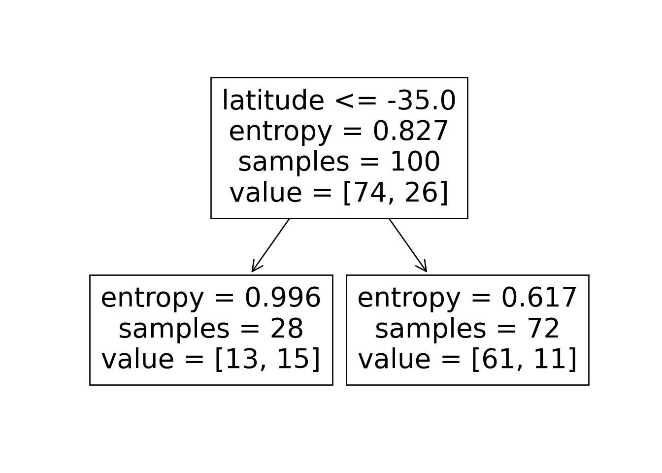

The Estimated Tree:

Performance:

Attaching package: 'arrow'

The following object is masked from 'package:lubridate':

    duration

The following object is masked from 'package:utils':

    timestamp

New names:
• `` -> `...1`

Rows: 100 Columns: 6
── Column specification ────────────────────────────────────────────────────────
Delimiter: ","
dbl (5): ...1, day_num, latitude, good_skiing, y_pred
lgl (1): correct

ℹ Use `spec()` to retrieve the full column specification for this data.
ℹ Specify the column types or set `show_col_types = FALSE` to quiet this message.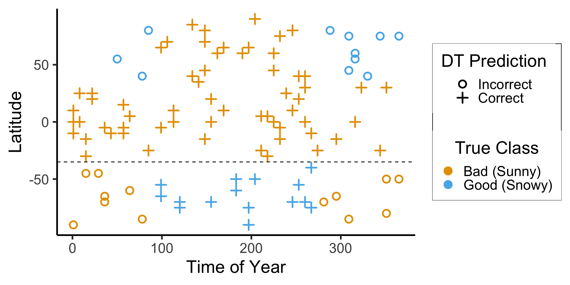

correct	n
FALSE	24
TRUE	76

\[ \begin{align*} \mathscr{L}(R_1) &= -\left[ \frac{13}{28}\log_2\left(\frac{13}{28}\right) + \frac{15}{28}\log_2\left(\frac{15}{28}\right) \right] \approx 0.996 \\ \mathscr{L}(R_2) &= -\left[ \frac{61}{72}\log_2\left(\frac{61}{72}\right) + \frac{11}{72}\log_2\left(\frac{11}{72}\right) \right] \approx 0.617 \\ %\mathscr{L}(R \rightarrow (R_1, R_2)) &= \Pr(x_i \in R_1)\mathscr{L}(R_1) + \Pr(x_i \in R_2)\mathscr{L}(R_2) \\ \mathscr{L}(R_1, R_2) &= \frac{28}{100}(0.996) + \frac{72}{100}(0.617) \approx 0.723 < 0.827~😻 \end{align*} \]

Continuous Values

• What if we replace binary labels with continuous values: in this case, cm of snow?

#format_snow <- function(x) sprintf('%.2f', x)
format_snow <- function(x) round(x, 2)
ski_sample['snowfall_str'] <- sapply(ski_sample$snowfall, format_snow)
#ski_df |> head()
#print(nrow(ski_df))
ggplot(ski_sample, aes(x=day, y=latitude, label=snowfall_str)) +
  geom_text(size = 6) +
  dsan_theme() +
  labs(
    x = "Time of Year",
    y = "Latitude",
    shape = "Good Skiing?"
  ) +
  scale_shape_manual(values=c(1, 3)) +
  scale_x_continuous(
    breaks=c(ymd('2023-01-01'), ymd('2023-02-01'), ymd('2023-03-01'), ymd('2023-04-01'), ymd('2023-05-01'), ymd('2023-06-01'), ymd('2023-07-01'), ymd('2023-08-01'), ymd('2023-09-01'), ymd('2023-10-01'), ymd('2023-11-01'), ymd('2023-12-01')),
    labels=c("Jan", "Feb", "Mar", "Apr", "May", "Jun", "Jul", "Aug", "Sep", "Oct", "Nov", "Dec")
  ) +
  scale_y_continuous(breaks=c(-90, -60, -30, 0, 30, 60, 90))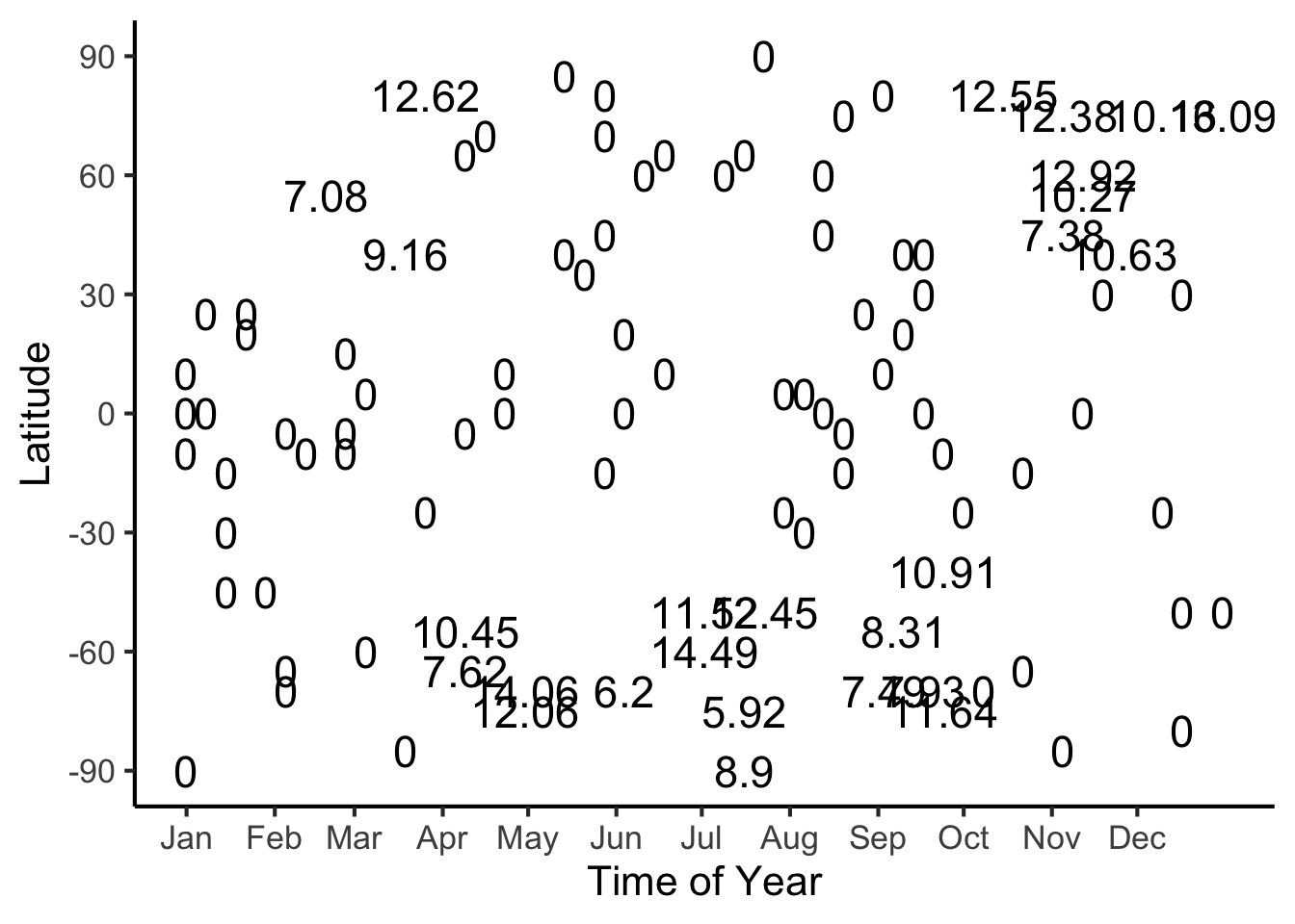

(Example adapted from CS229: Machine Learning, Stanford University)

Looking Towards Regression

• How could we make a decision tree to predict \(y\) from \(x\) for this data?

library(tidyverse)
library(latex2exp)
expr_pi2 <- TeX("$\\frac{\\pi}{2}$")
expr_pi <- TeX("$\\pi$")
expr_3pi2 <- TeX("$\\frac{3\\pi}{2}$")
expr_2pi <- TeX("$2\\pi$")
x_range <- 2 * pi
x_coords <- seq(0, x_range, by = x_range / 100)
num_x_coords <- length(x_coords)
data_df <- tibble(x = x_coords)
data_df <- data_df |> mutate(
  y_raw = sin(x),
  y_noise = rnorm(num_x_coords, 0, 0.15)
)
data_df <- data_df |> mutate(
  y = y_raw + y_noise
)
#y_coords <- y_raw_coords + y_noise
#y_coords <- y_raw_coords
#data_df <- tibble(x = x, y = y)
reg_tree_plot <- ggplot(data_df, aes(x=x, y=y)) +
  geom_point(size = g_pointsize / 2) +
  dsan_theme("half") +
  labs(
    x = "Feature",
    y = "Label"
  ) +
  geom_vline(
    xintercept = pi,
    linewidth = g_linewidth,
    linetype = "dashed"
  ) +
  scale_x_continuous(
    breaks=c(0,pi/2,pi,(3/2)*pi,2*pi),
    labels=c("0",expr_pi2,expr_pi,expr_3pi2,expr_2pi)
  )
reg_tree_plot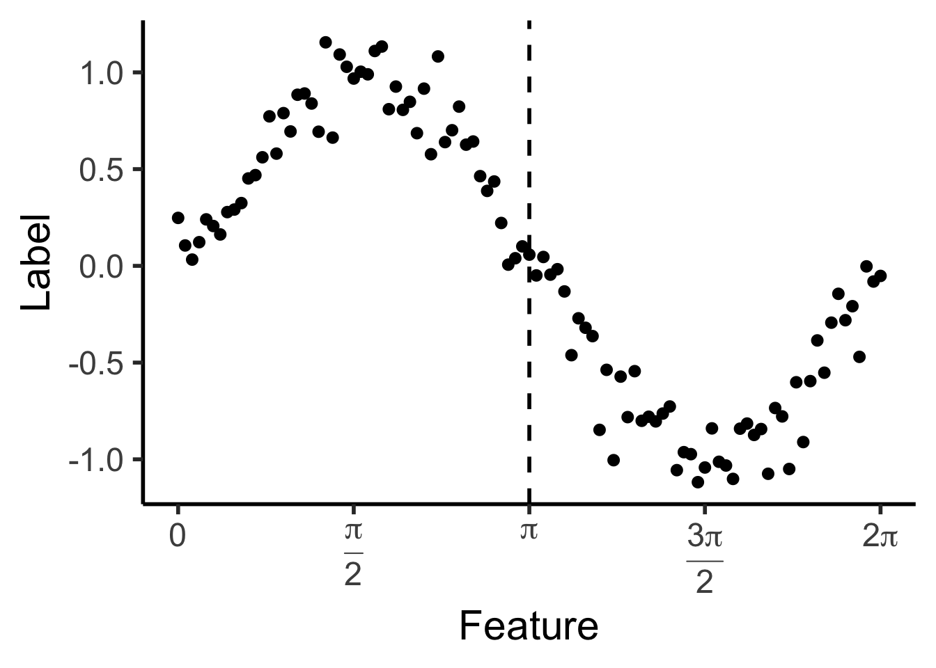

A Zero-Level Tree

• Trivial example: \(\widehat{y}(x) = 0\). How well does this do?

library(ggtext)
# x_lt_pi = data_df |> filter(x < pi)
# mean(x_lt_pi$y)
data_df <- data_df |> mutate(
  pred_sq_err0 = (y - 0)^2
)
mse0 <- mean(data_df$pred_sq_err0)
mse0_str <- sprintf("%.3f", mse0)
reg_tree_plot +
  geom_hline(
    yintercept = 0,
    color=cbPalette[1],
    linewidth = g_linewidth
  ) +
  geom_segment(
    aes(x=x, xend=x, y=0, yend=y)
  ) +
  geom_text(
    aes(x=(3/2)*pi, y=0.5, label=paste0("MSE = ",mse0_str)),
    size = 10,
    #box.padding = unit(c(2,2,2,2), "pt")
  )

Warning in geom_text(aes(x = (3/2) * pi, y = 0.5, label = paste0("MSE = ", : All aesthetics have length 1, but the data has 101 rows.
ℹ Please consider using `annotate()` or provide this layer with data containing
  a single row.

A One-Level Binary Tree

• Let’s introduce a single branch node:

\[ \widehat{y}(x) = \begin{cases} \phantom{-}\frac{2}{\pi} &\text{if }x < \pi, \\ -\frac{2}{\pi} &\text{otherwise.} \end{cases} \]

get_y_pred <- function(x) ifelse(x < pi, 2/pi, -2/pi)
data_df <- data_df |> mutate(
  pred_sq_err1 = (y - get_y_pred(x))^2
)
mse1 <- mean(data_df$pred_sq_err1)
mse1_str <- sprintf("%.3f", mse1)
decision_df <- tribble(
  ~x, ~xend, ~y, ~yend,
  0, pi, 2/pi, 2/pi,
  pi, 2*pi, -2/pi, -2/pi
)
reg_tree_plot +
  geom_segment(
    data=decision_df,
    aes(x=x, xend=xend, y=y, yend=yend),
    color=cbPalette[1],
    linewidth = g_linewidth
  ) +
  geom_segment(
    aes(x=x, xend=x, y=get_y_pred(x), yend=y)
  ) +
  geom_text(
    aes(x=(3/2)*pi, y=0.5, label=paste0("MSE = ",mse1_str)),
    size = 9,
    #box.padding = unit(c(2,2,2,2), "pt")
  )

Warning in geom_text(aes(x = (3/2) * pi, y = 0.5, label = paste0("MSE = ", : All aesthetics have length 1, but the data has 101 rows.
ℹ Please consider using `annotate()` or provide this layer with data containing
  a single row.

A One-Level Ternary Tree

• Now let’s allow three answers:

\[ \widehat{y}(x) = \begin{cases} \phantom{-}\frac{9}{4\pi} &\text{if }x < \frac{2\pi}{3}, \\ \phantom{-}0 &\text{if }\frac{2\pi}{3} \leq x \leq \frac{4\pi}{3} \\ -\frac{9}{4\pi} &\text{otherwise.} \end{cases} \]

cut1 <- (2/3) * pi
cut2 <- (4/3) * pi
pos_mean <- 9 / (4*pi)
get_y_pred <- function(x) ifelse(x < cut1, pos_mean, ifelse(x < cut2, 0, -pos_mean))
data_df <- data_df |> mutate(
  pred_sq_err1b = (y - get_y_pred(x))^2
)
mse1b <- mean(data_df$pred_sq_err1b)
mse1b_str <- sprintf("%.3f", mse1b)
decision_df <- tribble(
  ~x, ~xend, ~y, ~yend,
  0, (2/3)*pi, pos_mean, pos_mean,
  (2/3)*pi, (4/3)*pi, 0, 0,
  (4/3)*pi, 2*pi, -pos_mean, -pos_mean
)
reg_tree_plot +
  geom_segment(
    data=decision_df,
    aes(x=x, xend=xend, y=y, yend=yend),
    color=cbPalette[1],
    linewidth = g_linewidth
  ) +
  geom_segment(
    aes(x=x, xend=x, y=get_y_pred(x), yend=y)
  ) +
  geom_text(
    aes(x=(3/2)*pi, y=0.5, label=paste0("MSE = ",mse1b_str)),
    size = 9,
    #box.padding = unit(c(2,2,2,2), "pt")
  )

Warning in geom_text(aes(x = (3/2) * pi, y = 0.5, label = paste0("MSE = ", : All aesthetics have length 1, but the data has 101 rows.
ℹ Please consider using `annotate()` or provide this layer with data containing
  a single row.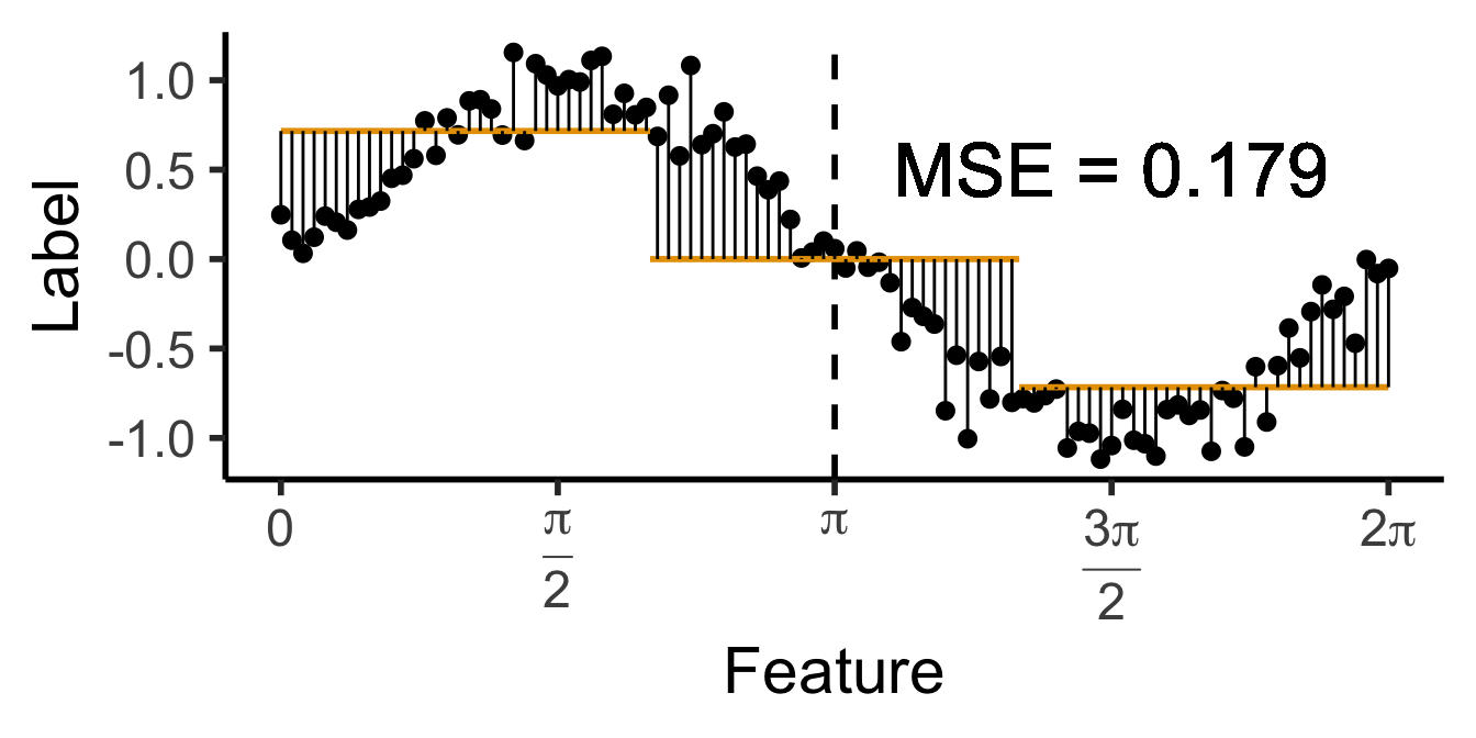

Another One-Level Ternary Tree

• Now let’s allow an uneven split:

\[ \widehat{y}(x) = \begin{cases} \phantom{-}0.695 &\text{if }x < (1-c)\pi, \\ \phantom{-}0 &\text{if }(1-c)\pi \leq x \leq (1+c)\pi \\ -0.695 &\text{otherwise,} \end{cases} \]

with \(c \approx 0.113\), gives us:

c <- 0.113
cut1 <- (1 - c) * pi
cut2 <- (1 + c) * pi
pos_mean <- 0.695
get_y_pred <- function(x) ifelse(x < cut1, pos_mean, ifelse(x < cut2, 0, -pos_mean))
data_df <- data_df |> mutate(
  pred_sq_err1b = (y - get_y_pred(x))^2
)
mse1b <- mean(data_df$pred_sq_err1b)
mse1b_str <- sprintf("%.3f", mse1b)
decision_df <- tribble(
  ~x, ~xend, ~y, ~yend,
  0, cut1, pos_mean, pos_mean,
  cut1, cut2, 0, 0,
  cut2, 2*pi, -pos_mean, -pos_mean
)
reg_tree_plot +
  geom_segment(
    data=decision_df,
    aes(x=x, xend=xend, y=y, yend=yend),
    color=cbPalette[1],
    linewidth = g_linewidth
  ) +
  geom_segment(
    aes(x=x, xend=x, y=get_y_pred(x), yend=y)
  ) +
  geom_text(
    aes(x=(3/2)*pi, y=0.5, label=paste0("MSE = ",mse1b_str)),
    size = 9,
    #box.padding = unit(c(2,2,2,2), "pt")
  )

Warning in geom_text(aes(x = (3/2) * pi, y = 0.5, label = paste0("MSE = ", : All aesthetics have length 1, but the data has 101 rows.
ℹ Please consider using `annotate()` or provide this layer with data containing
  a single row.

On to the Code!

• Scikit-learn has both DecisionTreeClassifier and DecisionTreeRegressor classes!

Regression Trees: Harder Task, Simpler Goal

• Last week we started with classification task (of good vs. bad skiing weather), to get a feel for how decision trees approach these tasks

• This week, for a deeper dive into the math/code, let’s start with regression. But why?

  • Despite the fact that the task itself is harder (have to guess an output \(\ell \in \mathbb{R}\) rather than \(\ell \in \{0, 1\}\)),
  • Our objective/goal is easier to define: given feature matrix \(\mathbf{X} = [\begin{smallmatrix}X_1 & \cdots & X_n\end{smallmatrix}]\) and labels \(\boldsymbol\ell = (\ell_1, \ldots, \ell_n)^\top\), find a function \(\widehat{f}\) which minimizes

  \[ \mathscr{L}_{\text{MSE}}\left(\widehat{f}~\right) = \sum_{i=1}^N \left(\widehat{f}(X_i) - \ell_i\right)^2 \]

• Once we’re comfortable with how to approach this regression task, we’ll move back to the classification task, where there is no longer a single “obvious” choice for the loss function \(\mathscr{L}\left(\widehat{f}~\right)\)

A Zero-Level Tree

• Trivial example: \(\widehat{y}(x) = 0\). (We ignore the feature value)
• How well does this do?

library(ggtext)
# x_lt_pi = data_df |> filter(x < pi)
# mean(x_lt_pi$y)
data_df <- data_df |> mutate(
  pred_sq_err0 = (y - 0)^2
)
mse0 <- mean(data_df$pred_sq_err0)
mse0_str <- sprintf("%.3f", mse0)
reg_tree_plot +
  geom_hline(
    yintercept = 0,
    color=cbPalette[1],
    linewidth = g_linewidth
  ) +
  geom_segment(
    aes(x=x, xend=x, y=0, yend=y)
  ) +
  geom_text(
    aes(x=(3/2)*pi, y=0.5, label=paste0("MSE = ",mse0_str)),
    size = 10,
    #box.padding = unit(c(2,2,2,2), "pt")
  )

Warning in geom_text(aes(x = (3/2) * pi, y = 0.5, label = paste0("MSE = ", : All aesthetics have length 1, but the data has 101 rows.
ℹ Please consider using `annotate()` or provide this layer with data containing
  a single row.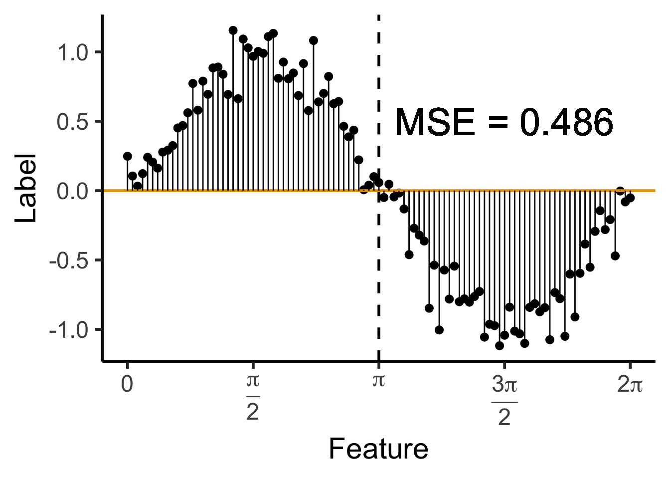

A One-Level Binary Tree

• Let’s introduce a single branch node:

\[ \widehat{y}(x) = \begin{cases} \phantom{-}\frac{2}{\pi} &\text{if }x < \pi, \\ -\frac{2}{\pi} &\text{otherwise.} \end{cases} \]

get_y_pred <- function(x) ifelse(x < pi, 2/pi, -2/pi)
data_df <- data_df |> mutate(
  pred_sq_err1 = (y - get_y_pred(x))^2
)
mse1 <- mean(data_df$pred_sq_err1)
mse1_str <- sprintf("%.3f", mse1)
decision_df <- tribble(
  ~x, ~xend, ~y, ~yend,
  0, pi, 2/pi, 2/pi,
  pi, 2*pi, -2/pi, -2/pi
)
reg_tree_plot +
  geom_segment(
    data=decision_df,
    aes(x=x, xend=xend, y=y, yend=yend),
    color=cbPalette[1],
    linewidth = g_linewidth
  ) +
  geom_segment(
    aes(x=x, xend=x, y=get_y_pred(x), yend=y)
  ) +
  geom_text(
    aes(x=(3/2)*pi, y=0.5, label=paste0("MSE = ",mse1_str)),
    size = 9,
    #box.padding = unit(c(2,2,2,2), "pt")
  )

Warning in geom_text(aes(x = (3/2) * pi, y = 0.5, label = paste0("MSE = ", : All aesthetics have length 1, but the data has 101 rows.
ℹ Please consider using `annotate()` or provide this layer with data containing
  a single row.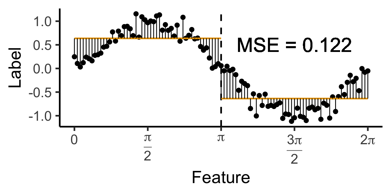

A One-Level Ternary Tree

• Now let’s allow three answers:

\[ \widehat{y}(x) = \begin{cases} \phantom{-}\frac{9}{4\pi} &\text{if }x < \frac{2\pi}{3}, \\ \phantom{-}0 &\text{if }\frac{2\pi}{3} \leq x \leq \frac{4\pi}{3} \\ -\frac{9}{4\pi} &\text{otherwise.} \end{cases} \]

cut1 <- (2/3) * pi
cut2 <- (4/3) * pi
pos_mean <- 9 / (4*pi)
get_y_pred <- function(x) ifelse(x < cut1, pos_mean, ifelse(x < cut2, 0, -pos_mean))
data_df <- data_df |> mutate(
  pred_sq_err1b = (y - get_y_pred(x))^2
)
mse1b <- mean(data_df$pred_sq_err1b)
mse1b_str <- sprintf("%.3f", mse1b)
decision_df <- tribble(
  ~x, ~xend, ~y, ~yend,
  0, (2/3)*pi, pos_mean, pos_mean,
  (2/3)*pi, (4/3)*pi, 0, 0,
  (4/3)*pi, 2*pi, -pos_mean, -pos_mean
)
reg_tree_plot +
  geom_segment(
    data=decision_df,
    aes(x=x, xend=xend, y=y, yend=yend),
    color=cbPalette[1],
    linewidth = g_linewidth
  ) +
  geom_segment(
    aes(x=x, xend=x, y=get_y_pred(x), yend=y)
  ) +
  geom_text(
    aes(x=(3/2)*pi, y=0.5, label=paste0("MSE = ",mse1b_str)),
    size = 9,
    #box.padding = unit(c(2,2,2,2), "pt")
  )

Warning in geom_text(aes(x = (3/2) * pi, y = 0.5, label = paste0("MSE = ", : All aesthetics have length 1, but the data has 101 rows.
ℹ Please consider using `annotate()` or provide this layer with data containing
  a single row.

Another One-Level Ternary Tree

• Now let’s allow an uneven split:

\[ \widehat{y}(x) = \begin{cases} \phantom{-}0.695 &\text{if }x < (1-c)\pi, \\ \phantom{-}0 &\text{if }(1-c)\pi \leq x \leq (1+c)\pi \\ -0.695 &\text{otherwise,} \end{cases} \]

with \(c \approx 0.113\), gives us:

c <- 0.113
cut1 <- (1 - c) * pi
cut2 <- (1 + c) * pi
pos_mean <- 0.695
get_y_pred <- function(x) ifelse(x < cut1, pos_mean, ifelse(x < cut2, 0, -pos_mean))
data_df <- data_df |> mutate(
  pred_sq_err1b = (y - get_y_pred(x))^2
)
mse1b <- mean(data_df$pred_sq_err1b)
mse1b_str <- sprintf("%.3f", mse1b)
decision_df <- tribble(
  ~x, ~xend, ~y, ~yend,
  0, cut1, pos_mean, pos_mean,
  cut1, cut2, 0, 0,
  cut2, 2*pi, -pos_mean, -pos_mean
)
reg_tree_plot +
  geom_segment(
    data=decision_df,
    aes(x=x, xend=xend, y=y, yend=yend),
    color=cbPalette[1],
    linewidth = g_linewidth
  ) +
  geom_segment(
    aes(x=x, xend=x, y=get_y_pred(x), yend=y)
  ) +
  geom_text(
    aes(x=(3/2)*pi, y=0.5, label=paste0("MSE = ",mse1b_str)),
    size = 9,
    #box.padding = unit(c(2,2,2,2), "pt")
  )

Warning in geom_text(aes(x = (3/2) * pi, y = 0.5, label = paste0("MSE = ", : All aesthetics have length 1, but the data has 101 rows.
ℹ Please consider using `annotate()` or provide this layer with data containing
  a single row.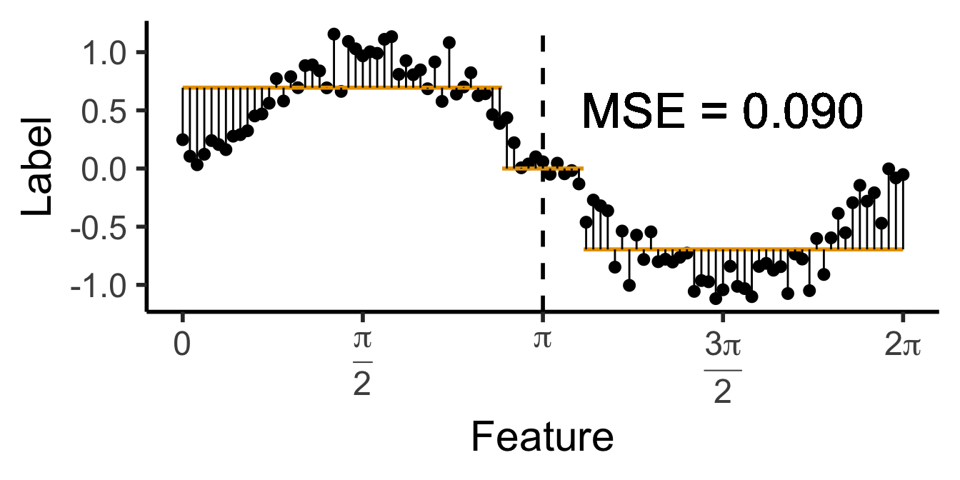

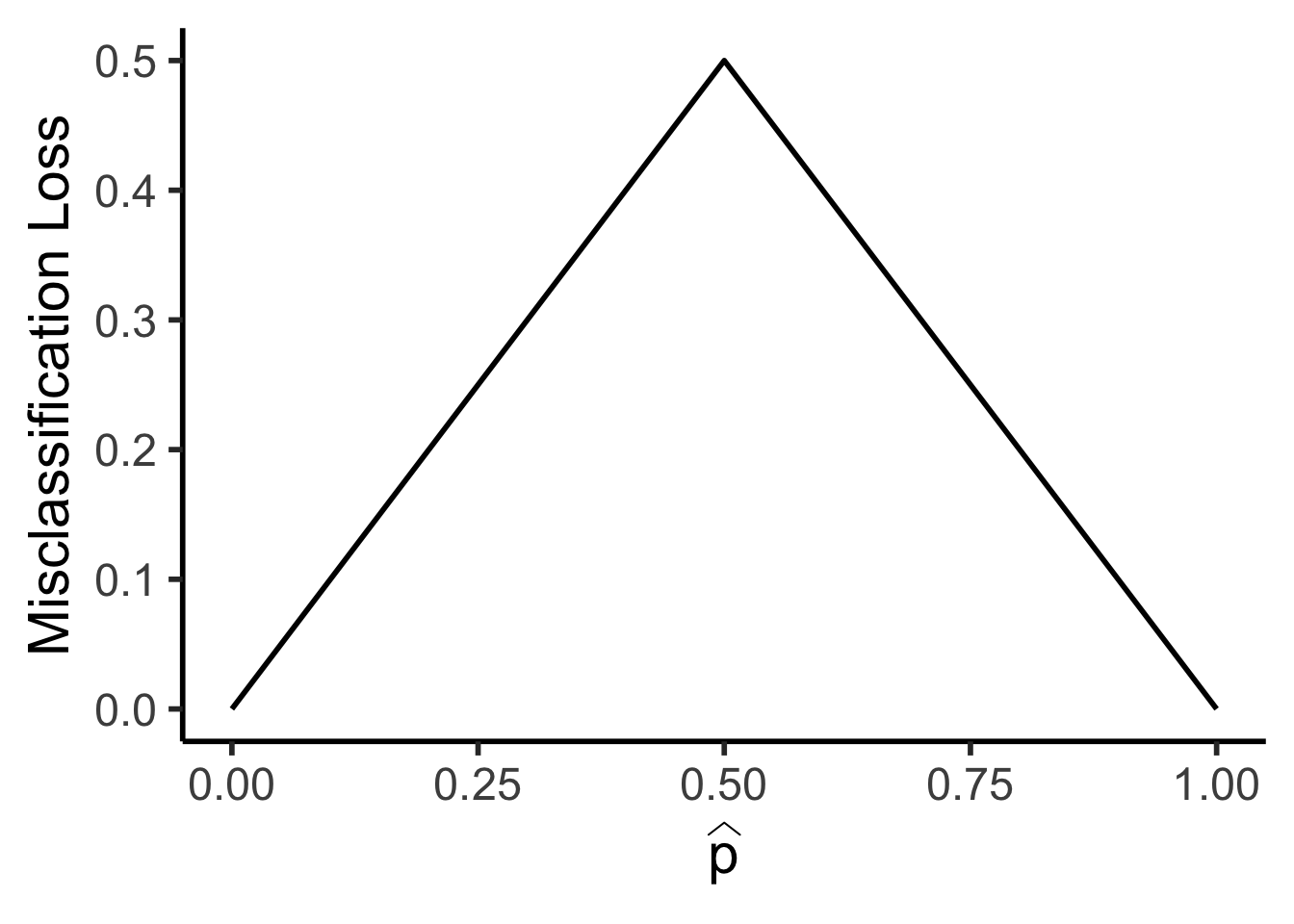
Onto Classification

• We’d like to carry out a similar process for classification tasks: (1) try a split of the full space into \(K\) sub-regions, then (2) evaluate the split based on how much it reduces uncertainty
• But, the discreteness of labels in this case means we cannot just “import” MSE as our loss function
• For example, if the true class for a datapoint \(i\) is \(\ell_i = 1\), is a guess \(\widehat{\ell} = 3\) “twice as wrong” as \(\widehat{\ell} = 2\)?
• So, let’s brainstorm a discrete loss function

Getting Closer

• Your first instinct might be to choose the misclassification rate, the proportion of points in region \(R\) that we are misclassifying if we guess the most-common class:

\[ \mathscr{L}_{MC}(R) = 1 - \widehat{p}_{R} \]

• The shape of this function, however, gives us a hint as to why we may want to choose a different function:

library(tidyverse)
library(latex2exp)
my_mc <- function(p) 0.5 - abs(0.5 - p)
x_vals <- seq(0, 1, 0.01)
mc_vals <- sapply(x_vals, my_mc)
phat_label <- TeX('$\\widehat{p}$')
data_df <- tibble(x=x_vals, loss_mc=mc_vals)
ggplot(data_df, aes(x=x, y=loss_mc)) +
  geom_line(linewidth = g_linewidth) +
  dsan_theme("half") +
  labs(
    x = phat_label,
    y = "Misclassification Loss"
  )

Using Misclassification Loss to Choose a Split

• Given a parent region \(R_P\), we’re trying to choose a split into subregions \(R_1\) and \(R_2\) which will decrease the loss: \(\frac{|R_1|}{|R_P|}\mathscr{L}(R_1) + \frac{|R_2|}{|R_P|}\mathscr{L}(R_2) < \mathscr{L}(R_P)\)
• But what happens when we use misclassification loss to “judge” a split?

• Tl;dr this doesn’t “detect” when we’ve reduced uncertainty
• But we do have a function that was constructed to measure uncertainty!

Using Entropy to Choose a Split

Is There Another Option?

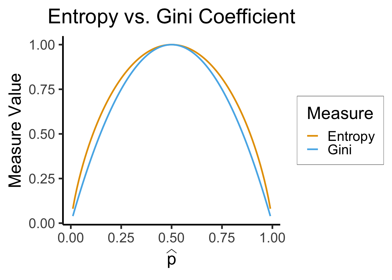
\[ \mathscr{L}_{\text{Ent}}(\widehat{p}) = -\sum_{i=1}^K \widehat{p}_k\log_2(\widehat{p}_k) \]

\[ \mathscr{L}_{\text{Gini}}(\widehat{p}) = -\sum_{i=1}^K \widehat{p}_k(1-\widehat{p}_k) \]

library(tidyverse)
library(latex2exp)
phat_label <- TeX('$\\widehat{p}')
my_ent <- function(p) -(p*log2(p) + (1-p)*log2(1-p))
my_gini <- function(p) 4*p*(1-p)
x_vals <- seq(0.01, 0.99, 0.01)
ent_vals <- sapply(x_vals, my_ent)
ent_df <- tibble(x=x_vals, y=ent_vals, Measure="Entropy")
gini_vals <- sapply(x_vals, my_gini)
gini_df <- tibble(x=x_vals, y=gini_vals, Measure="Gini")
data_df <- bind_rows(ent_df, gini_df)
ggplot(data=data_df, aes(x=x, y=y, color=Measure)) +
  geom_line(linewidth = g_linewidth) +
  dsan_theme("half") +
  scale_color_manual(values=c(cbPalette[1], cbPalette[2])) +
  labs(
    x = phat_label,
    y = "Measure Value",
    title = "Entropy vs. Gini Coefficient"
  )

The Space of All Decision Trees

• Why can’t we just try all possible decision trees, and choose the one with minimum loss? Consider a case with just \(N = 1\) binary feature, \(F_1 \in \{0, 1\}\):

\(T_0\): Predict \(\ell = 0\) always (regardless of value of \(F_1\))

\(T_1\): Predict \(\ell = 1\) always (regardless of value of \(F_1\))

\(T_2\): Predict \(\ell = 1\) when \(F_1 = 1\), otherwise \(\ell = 0\)

\(T_3\): Predict \(\ell = 1\) when \(F_1 = 0\), otherwise \(\ell = 1\)

Decision Trees \(\leftrightarrow\) Binary Functions

• Possible binary decision trees over \(N\) binary features \(\leftrightarrow\) possible binary functions mapping all \(2^N\) possible inputs to an output \(\widehat{\ell} \in \{0,1\}\)
• That is, all functions \(f: 2^N \rightarrow \{0,1\}\). There are \(2^{2^N}\) such functions 😵‍💫
• Previous slide:
  • \(T_0 = \{(f_1 = 0) \rightarrow 0, (f_1 = 1) \rightarrow 0\}\)
  • \(T_1 = \{(f_1 = 0) \rightarrow 1, (f_1 = 1) \rightarrow 1\}\)
  • \(T_2 = \{(f_1 = 0) \rightarrow 0, (f_1 = 1) \rightarrow 1\}\)
  • \(T_3 = \{(f_1 = 0) \rightarrow 1, (f_1 = 1) \rightarrow 0\}\)
• With \(N = 2\) binary features, each tree would choose a possible decision for inputs \((f_1 = 0, f_2 = 0)\), \((f_1 = 0, f_2 = 1)\), \((f_1 = 1, f_2 = 0)\), \((f_1 = 1, f_2 = 1)\)
• Possible binary DTs over \(N\) ternary (3-class) features \(\leftrightarrow\) map all \(3^N\) inputs to output \(\widehat{\ell} \in \{0, 1\} \implies 2^{3^N}\) ternary DTs… Ternary DTs, \(N\) ternary features \(\implies\) \(3^{3^N}\) DTs

So What Do We Do Instead?

• We get greedy!
• Start from the top of the tree, and at each level, choose feature \(j^*\) and splitpoint \(s^*\) as solution to:

\[ (j^*, s^*) = \argmax_{j, s}\left[ \mathscr{L}(R_1(j,s)) + \mathscr{L}(R_2(j,s)) \right], \]

where

\[ R_1(j, s) = \{X \mid X_j < s\}, \; R_2(j, s) = \{X \mid X_j \geq s\}. \]

Back to the Skiing Example

library(tidyverse)
library(lubridate)
set.seed(5001)
sample_size <- 100
day <- seq(ymd('2023-01-01'),ymd('2023-12-31'),by='weeks')
lat_bw <- 5
latitude <- seq(-90, 90, by=lat_bw)
ski_df <- expand_grid(day, latitude)
ski_df <- tibble::rowid_to_column(ski_df, var='obs_id')
#ski_df |> head()
# Data-generating process
lat_cutoff <- 35
ski_df <- ski_df |> mutate(
  near_equator = abs(latitude) <= lat_cutoff,
  northern = latitude > lat_cutoff,
  southern = latitude < -lat_cutoff,
  first_3m = day < ymd('2023-04-01'),
  last_3m = day >= ymd('2023-10-01'),
  middle_6m = (day >= ymd('2023-04-01')) & (day < ymd('2023-10-01')),
  snowfall = 0
)
# Update the non-zero sections
mu_snow <- 10
sd_snow <- 2.5
# How many northern + first 3 months
num_north_first_3 <- nrow(ski_df[ski_df$northern & ski_df$first_3m,])
ski_df[ski_df$northern & ski_df$first_3m, 'snowfall'] = rnorm(num_north_first_3, mu_snow, sd_snow)
# Northerns + last 3 months
num_north_last_3 <- nrow(ski_df[ski_df$northern & ski_df$last_3m,])
ski_df[ski_df$northern & ski_df$last_3m, 'snowfall'] = rnorm(num_north_last_3, mu_snow, sd_snow)
# How many southern + middle 6 months
num_south_mid_6 <- nrow(ski_df[ski_df$southern & ski_df$middle_6m,])
ski_df[ski_df$southern & ski_df$middle_6m, 'snowfall'] = rnorm(num_south_mid_6, mu_snow, sd_snow)
# And collapse into binary var
ski_df['good_skiing'] = ski_df$snowfall > 0
# This converts day into an int
ski_df <- ski_df |> mutate(
  day_num = lubridate::yday(day)
)
#print(nrow(ski_df))
ski_sample <- ski_df |> slice_sample(n = sample_size)
ski_sample |> write_csv("assets/ski.csv")
month_vec <- c(ymd('2023-01-01'), ymd('2023-02-01'), ymd('2023-03-01'), ymd('2023-04-01'), ymd('2023-05-01'), ymd('2023-06-01'), ymd('2023-07-01'), ymd('2023-08-01'), ymd('2023-09-01'), ymd('2023-10-01'), ymd('2023-11-01'), ymd('2023-12-01'))
month_labels <- c("Jan", "Feb", "Mar", "Apr", "May", "Jun", "Jul", "Aug", "Sep", "Oct", "Nov", "Dec")
lat_vec <- c(-90, -60, -30, 0, 30, 60, 90)
ggplot(
  ski_sample,
  aes(
    x=day,
    y=latitude,
    #shape=good_skiing,
    color=good_skiing
  )) +
  geom_point(
    size = g_pointsize / 1.5,
    #stroke=1.5
  ) +
  dsan_theme() +
  labs(
    x = "Time of Year",
    y = "Latitude",
    shape = "Good Skiing?"
  ) +
  scale_shape_manual(name="Good Skiing?", values=c(1, 3)) +
  scale_color_manual(name="Good Skiing?", values=c(cbPalette[1], cbPalette[2]), labels=c("No (Sunny)","Yes (Snowy)")) +
  scale_x_continuous(
    breaks=c(month_vec,ymd('2024-01-01')),
    labels=c(month_labels,"Jan")
  ) +
  scale_y_continuous(breaks=lat_vec)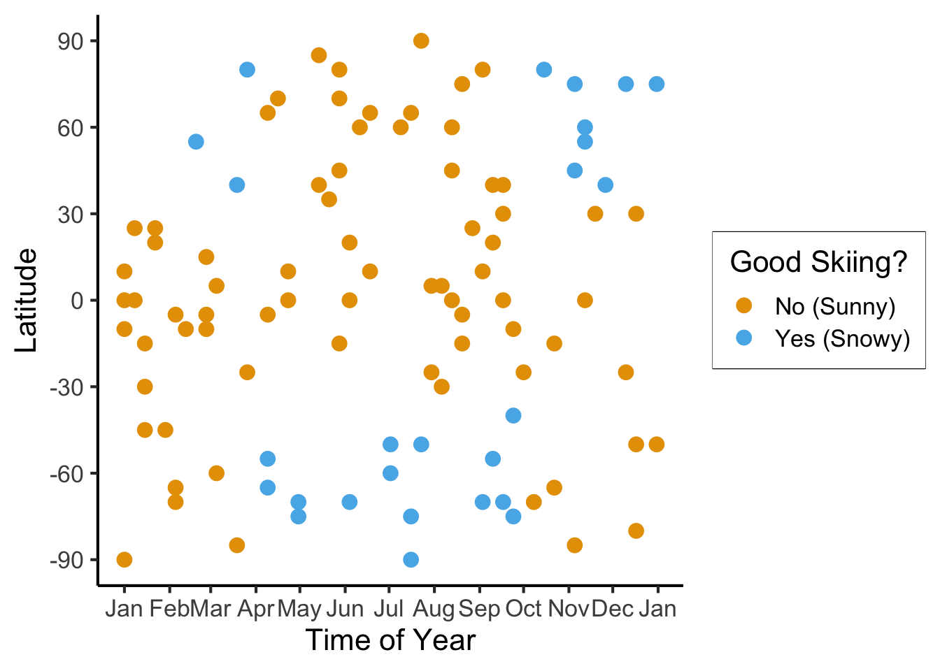

(Example adapted from CS229: Machine Learning, Stanford University)

The Parent Region

• Starting out: no splits at all, so that \(R = \{X_i \mid X_i \in \mathbf{X} \}\)
• So we just guess most frequent class in the dataset: bad skiing

ski_sample |> count(good_skiing)

good_skiing	n
FALSE	74
TRUE	26

• This gives us \(\Pr(\text{Correct Guess} \mid \text{Guess Bad}) = 0.74\)
• Since we’re not splitting the region up at all (yet), the entropy is just

\[ \mathscr{L}(R_i) = -[(0.74)\log_2(0.74) + (0.26)\log_2(0.26)] \approx 0.8267 \]

Judging Split Options

Given that \(\mathscr{L}(R_P) \approx 0.9427\), let’s think through two choices for the first split:

ski_sample <- ski_sample |> mutate(
  lat_lt_n425 = latitude < -42.5
)
r1a <- ski_sample |> filter(lat_lt_n425) |> summarize(
  good_skiing = sum(good_skiing),
  total = n()
) |> mutate(region = "R1(A)", .before=good_skiing)
r2a <- ski_sample |> filter(lat_lt_n425 == FALSE) |> summarize(
  good_skiing = sum(good_skiing),
  total = n()
) |> mutate(region = "R2(A)", .before=good_skiing)
choice_a_df <- bind_rows(r1a, r2a)
choice_a_df
ski_sample <- ski_sample |> mutate(
  month_lt_oct = day < ymd('2023-10-01')
)
r1b <- ski_sample |> filter(month_lt_oct) |> summarize(
  good_skiing = sum(good_skiing),
  total = n()
) |> mutate(region = "R1(B)", .before=good_skiing)
r2b <- ski_sample |> filter(month_lt_oct == FALSE) |> summarize(
  good_skiing = sum(good_skiing),
  total = n()
) |> mutate(region = "R2(B)", .before=good_skiing)
choice_b_df <- bind_rows(r1b, r2b)
choice_b_df

\((f^A = \text{Latitude}\), \(s^A = -42.5)\)

\[ \begin{align*} R_1^A &= \{X_i \mid X_{i,\text{lat}} < -42.5\} \\ R_2^A &= \{X_i \mid X_{i,\text{lat}} \geq -42.5\} \end{align*} \]

region	good_skiing	total
R1(A)	14	27
R2(A)	12	73

\[ \begin{align*} \mathscr{L}(R_1^A) &= -\mkern-4mu\left[ \frac{21}{32}\log_2\frac{21}{32} + \frac{11}{32}\log_2\frac{11}{32} \right] \approx 0.9284 \\ \mathscr{L}(R_2^A) &= -\mkern-4mu\left[ \frac{15}{68}\log_2\frac{15}{68} + \frac{53}{68}\log_2\frac{53}{68}\right] \approx 0.7612 \\ \implies \mathscr{L}(A) &= \frac{32}{100}(0.9284) + \frac{68}{100}(0.7612) \approx 0.8147 % < 0.9427 \end{align*} \]

 

\((f^B = \text{Month}, s^B = \text{October})\)

\[ \begin{align*} R_1^B &= \{X_i \mid X_{i,\text{month}} < \text{October}\} \\ R_2^B &= \{X_i \mid X_{i,\text{month}} \geq \text{October}\} \end{align*} \]

region	good_skiing	total
R1(B)	18	80
R2(B)	8	20

\[ \begin{align*} \mathscr{L}(R_1^B) &= -\mkern-4mu\left[ \frac{28}{75}\log_2\frac{28}{75} + \frac{47}{75}\log_2\frac{47}{75}\right] \approx 0.9532 \\ \mathscr{L}(R_2^B) &= -\mkern-4mu\left[ \frac{8}{25}\log_2\frac{8}{25} + \frac{17}{25}\log_2\frac{17}{25} \right] \approx 0.9044 \\ \implies \mathscr{L}(B) &= \frac{75}{100}(0.9532) + \frac{25}{100}(0.9044) \approx 0.941 \end{align*} \]

• Notice: \(\mathscr{L}(A)\), \(\mathscr{L}(B)\) both \(< \mathscr{L}(R_P)\). But \(\mathscr{L}(R_P) - \mathscr{L}(A) = 0.128\), \(\mathscr{L}(R_P) - \mathscr{L}(B) = 0.0017\). \(B\) decreases our uncertainty more than \(A\), given \(R_P\).

When Do We Stop?

• Option 1: Stop when all nodes are pure; there is no uncertainty left
  • Pros: Perfect training accuracy!
  • Cons: The definition of overfitting
• Option 2: Manually restrict the number of levels, via a hyperparameter (could be max_levels, or min_samples_leaf)
• Option 3: Prune the tree using heuristic methods

Random Forests

The Wisdom of Crowds

• Imagine you’re assembling a darts team. You can choose a team of 4 from among the following 8 players:

Player	Skill
Larry “Lefty” Lechuga	Always hits 5cm left of bullseye
Rico Righty	Always hits 5cm right of bullseye
Lil Uppy Vert	Always hits 5cm above bullseye
Inconsistent Inkyung	Hits bullseye 50% of time, other 50% hits random point
Diagonal Dave	Always hits 5cm above right of bullseye
Dobert Downy Jr.	Always hits 5cm below bullseye
Gregor “the GOAT” Gregorsson	Hits bullseye 99.9% of time, other 0.1% hits random point
Craig	Top 25 Craigs of 2023

Your Opponents

High Variance, Low Bias

The Wisdom of Sheep

• Unfortunately, the “wisdom of crowds” phenomenon only works if everyone in the crowd is unable to communicate
• The minute people tasked with making decisions as a group begin to communicate (long story short), they begin to follow charismatic leaders , and the effect goes away (biases no longer cancel out)
• The takeaway for effectively training random forests: ensure that each tree has a separate (ideally orthogonal) slice of the full dataset, and has to infer labels from only that slice!

Bagging and Boosting

Decision Trees: What Now?

• We have a dataset and a decision tree… now what?
• If our only goal is interpretability, we’re done
• If we want to increase accuracy/efficiency, however, we can do better!

Bootstrapped Trees

Making up for Lost Interpretability

• While we no longer have a nice single tree structure, we can still “back out” the most important features!
• Basic idea: for importance of feature \(j\), loop over all subtrees, and look at the average decrease in uncertainty when a tree splits on feature \(j\)

Doing Even Better

• Issue: Each bootstrapped tree will be highly correlated
• If there is one extremely strong signal (think of the RateMyProfessors example!), associated with one (or a few) feature(s), all of the trees will focus on that feature
• How can we ensure that some trees pick up on more subtle signals within the dataset?

Decorrelating Trees

• Long story short: give each subtree only a subset of the features, of size \(M_i \approx \sqrt{M}\)
• Can prove that:
  • Smaller subsets \(\implies\) too much uncorrelated info to aggregate
  • Larger subsets \(\implies\) trees become correlated

But Wait…

• We’re giving each subtree a portion of the features, hoping that each one picks up on some important “sub-signal” in the data
• Instead of hoping, why don’t we make sure that each subtree is tasked with explaining the so-far-unexplained variation?
• Enter boosting 😎

Boosting

• Rather than giving each subtree a random subset of features, grow trees sequentially! Ask each subtree to explain remaining unexplained variance from previous step
• Step 1: \(\widehat{f}_1(X)\) = DT for \(X \rightarrow Y\)
• Step \(t+1\): \(\widehat{f}_{t+1}(X)\) = DT for \(X \rightarrow \left(\widehat{f}_t(X) - Y\right)\)

library(ggtext)
# x_lt_pi = data_df |> filter(x < pi)
# mean(x_lt_pi$y)
data_df <- data_df |> mutate(
  pred_sq_err0 = (y - 0)^2
)
mse0 <- mean(data_df$pred_sq_err0)
mse0_str <- sprintf("%.3f", mse0)
reg_tree_plot +
  geom_hline(
    yintercept = 0,
    color=cbPalette[1],
    linewidth = g_linewidth
  ) +
  geom_segment(
    aes(x=x, xend=x, y=0, yend=y)
  ) +
  geom_text(
    aes(x=(3/2)*pi, y=0.5, label=paste0("MSE = ",mse0_str)),
    size = 10,
    #box.padding = unit(c(2,2,2,2), "pt")
  )
get_y_pred <- function(x) ifelse(x < pi, 2/pi, -2/pi)
data_df <- data_df |> mutate(
  pred_sq_err1 = (y - get_y_pred(x))^2
)
mse1 <- mean(data_df$pred_sq_err1)
mse1_str <- sprintf("%.3f", mse1)
decision_df <- tribble(
  ~x, ~xend, ~y, ~yend,
  0, pi, 2/pi, 2/pi,
  pi, 2*pi, -2/pi, -2/pi
)
reg_tree_plot +
  geom_segment(
    data=decision_df,
    aes(x=x, xend=xend, y=y, yend=yend),
    color=cbPalette[1],
    linewidth = g_linewidth
  ) +
  geom_segment(
    aes(x=x, xend=x, y=get_y_pred(x), yend=y)
  ) +
  geom_text(
    aes(x=(3/2)*pi, y=0.5, label=paste0("MSE = ",mse1_str)),
    size = 9,
    #box.padding = unit(c(2,2,2,2), "pt")
  )

1. Original data

Warning in geom_text(aes(x = (3/2) * pi, y = 0.5, label = paste0("MSE = ", : All aesthetics have length 1, but the data has 101 rows.
ℹ Please consider using `annotate()` or provide this layer with data containing
  a single row.

2. One-level DT

Warning in geom_text(aes(x = (3/2) * pi, y = 0.5, label = paste0("MSE = ", : All aesthetics have length 1, but the data has 101 rows.
ℹ Please consider using `annotate()` or provide this layer with data containing
  a single row.

Appendix: Covariance Matrix Magic

• For those interested (skipping over lots of matrix math): say you have a 2D covariance matrix \(\mathbf{\Sigma}\) with eigensystem \((\lambda_1, \mathbf{x}_1), (\lambda_2, \mathbf{x}_2)\)
• You can obtain a new covariance matrix \(\mathbf{\Sigma}'\) which has the same eigenvalues as \(\mathbf{\Sigma}\) but has eigenvectors \(\mathbf{x}'_1\) and \(\mathbf{x}'_2\), so long as these two eigenvectors are orthogonal.
• Example: you want to retain the eigenvalues \(\lambda_1 = 3\) and \(\lambda_2 = 1\) from the quiz-review slides, but want the data’s first principal component to be \(\mathbf{x}'_1 = (2,1)^\top\) and its second principal component to be \(\mathbf{x}'_2 = (-1,2)^\top\).
• By constructing the Eigenmatrix \(\mathbf{V} = \left[\begin{smallmatrix} \mathbf{x}'_1 & \mathbf{x}'_2\end{smallmatrix}\right]\) (the matrix whose columns are \(\mathbf{x}'_1\) and \(\mathbf{x}'_2\)), we can obtain \(\mathbf{\Sigma}'\) by computing:

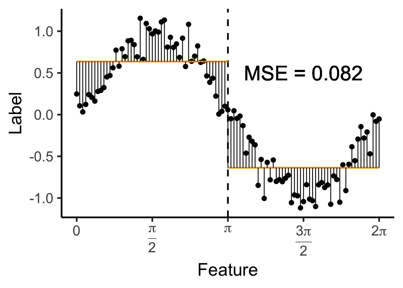
\[ \mathbf{\Sigma}' = \mathbf{V}\mathbf{\Sigma}\mathbf{V}^{-1}. \]

• (Exercise: recreate the plot from the earlier PCA slides, but with these desired first and second principal components! See here for a deeper dive into why this works!)

References