Week 11: Random Forests
DSAN 5000: Data Science and Analytics
Thursday, November 14, 2024
How Are They Built?
- Example: we find ourselves at some point on the globe, at some time during the year, and we’re trying to see whether this point+time are good for skiing
Code
library(tidyverse)
library(lubridate)
set.seed(5001)
sample_size <- 100
day <- seq(ymd('2023-01-01'),ymd('2023-12-31'),by='weeks')
lat_bw <- 5
latitude <- seq(-90, 90, by=lat_bw)
ski_df <- expand_grid(day, latitude)
#ski_df |> head()
# Data-generating process
lat_cutoff <- 35
ski_df <- ski_df |> mutate(
  near_equator = abs(latitude) <= lat_cutoff,
  northern = latitude > lat_cutoff,
  southern = latitude < -lat_cutoff,
  first_3m = day < ymd('2023-04-01'),
  last_3m = day >= ymd('2023-10-01'),
  middle_6m = (day >= ymd('2023-04-01')) & (day < ymd('2023-10-01')),
  snowfall = 0
)
# Update the non-zero sections
mu_snow <- 10
sd_snow <- 2.5
# How many northern + first 3 months
num_north_first_3 <- nrow(ski_df[ski_df$northern & ski_df$first_3m,])
ski_df[ski_df$northern & ski_df$first_3m, 'snowfall'] = rnorm(num_north_first_3, mu_snow, sd_snow)
# Northerns + last 3 months
num_north_last_3 <- nrow(ski_df[ski_df$northern & ski_df$last_3m,])
ski_df[ski_df$northern & ski_df$last_3m, 'snowfall'] = rnorm(num_north_last_3, mu_snow, sd_snow)
# How many southern + middle 6 months
num_south_mid_6 <- nrow(ski_df[ski_df$southern & ski_df$middle_6m,])
ski_df[ski_df$southern & ski_df$middle_6m, 'snowfall'] = rnorm(num_south_mid_6, mu_snow, sd_snow)
# And collapse into binary var
ski_df['good_skiing'] = ski_df$snowfall > 0
# This converts day into an int
ski_df <- ski_df |> mutate(
  day_num = lubridate::yday(day)
)
#print(nrow(ski_df))
ski_sample <- ski_df |> slice_sample(n = sample_size)
ski_sample |> write_csv("assets/ski.csv")
ggplot(
  ski_sample,
  aes(
    x=day,
    y=latitude,
    #shape=good_skiing,
    color=good_skiing
  )) +
  geom_point(
    size = g_pointsize / 1.5,
    #stroke=1.5
  ) +
  dsan_theme() +
  labs(
    x = "Time of Year",
    y = "Latitude",
    shape = "Good Skiing?"
  ) +
  scale_shape_manual(name="Good Skiing?", values=c(1, 3)) +
  scale_color_manual(name="Good Skiing?", values=c(cbPalette[1], cbPalette[2]), labels=c("No (Sunny)","Yes (Snowy)")) +
  scale_x_continuous(
    breaks=c(ymd('2023-01-01'), ymd('2023-02-01'), ymd('2023-03-01'), ymd('2023-04-01'), ymd('2023-05-01'), ymd('2023-06-01'), ymd('2023-07-01'), ymd('2023-08-01'), ymd('2023-09-01'), ymd('2023-10-01'), ymd('2023-11-01'), ymd('2023-12-01')),
    labels=c("Jan", "Feb", "Mar", "Apr", "May", "Jun", "Jul", "Aug", "Sep", "Oct", "Nov", "Dec")
  ) +
  scale_y_continuous(breaks=c(-90, -60, -30, 0, 30, 60, 90))
(Example adapted from CS229: Machine Learning, Stanford University)
Scikit-Learn: Growing the Tree
Code
import json
import pandas as pd
import numpy as np
import sklearn
from sklearn.tree import DecisionTreeClassifier
sklearn.set_config(display='text')
ski_df = pd.read_csv("assets/ski.csv")
ski_df['good_skiing'] = ski_df['good_skiing'].astype(int)
X = ski_df[['day_num', 'latitude']]
y = ski_df['good_skiing']
dtc = DecisionTreeClassifier(
  max_depth = 1,
  criterion = "entropy",
  random_state=5001
)
dtc.fit(X, y);
y_pred = pd.Series(dtc.predict(X), name="y_pred")
result_df = pd.concat([X,y,y_pred], axis=1)
result_df['correct'] = result_df['good_skiing'] == result_df['y_pred']
result_df.to_csv("assets/ski_predictions.csv")
sklearn.tree.plot_tree(dtc, feature_names = X.columns)
n_nodes = dtc.tree_.node_count
children_left = dtc.tree_.children_left
children_right = dtc.tree_.children_right
feature = dtc.tree_.feature
feat_index = feature[0]
feat_name = X.columns[feat_index]
thresholds = dtc.tree_.threshold
feat_threshold = thresholds[0]
#print(f"Feature: {feat_name}\nThreshold: <= {feat_threshold}")
values = dtc.tree_.value
#print(values)
dt_data = {
  'feat_index': feat_index,
  'feat_name': feat_name,
  'feat_threshold': feat_threshold
}
dt_df = pd.DataFrame([dt_data])
dt_df.to_feather('assets/ski_dt.feather')
library(tidyverse)
library(arrow)
# Load the dataset
ski_result_df <- read_csv("assets/ski_predictions.csv")
# Load the DT info
dt_df <- read_feather("assets/ski_dt.feather")
# Here we only have one value, so just read that
# value directly
lat_thresh <- dt_df$feat_threshold
ggplot(ski_result_df, aes(x=day_num, y=latitude, color=factor(good_skiing), shape=correct)) +
  geom_point(
    size = g_pointsize / 1.5,
    stroke = 1.5
  ) +
  geom_hline(
    yintercept = lat_thresh,
    linetype = "dashed"
  ) +
  dsan_theme("half") +
  labs(
    x = "Time of Year",
    y = "Latitude",
    color = "True Class",
    #shape = "Correct?"
  ) +
  scale_shape_manual("DT Prediction", values=c(1,3), labels=c("Incorrect","Correct")) +
  scale_color_manual("True Class", values=c(cbPalette[1], cbPalette[2]), labels=c("Bad (Sunny)","Good (Snowy)"))
ski_result_df |> count(correct)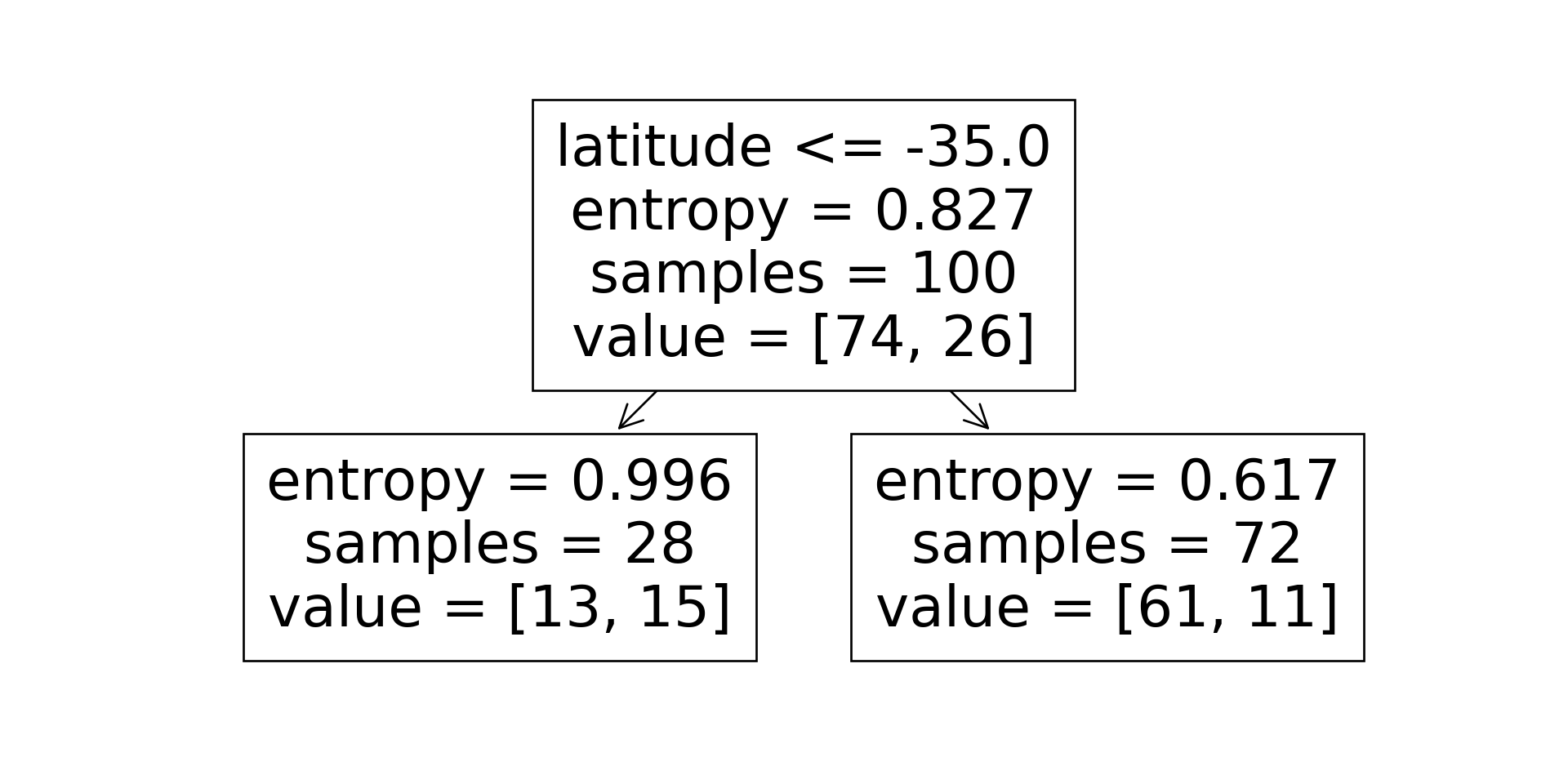
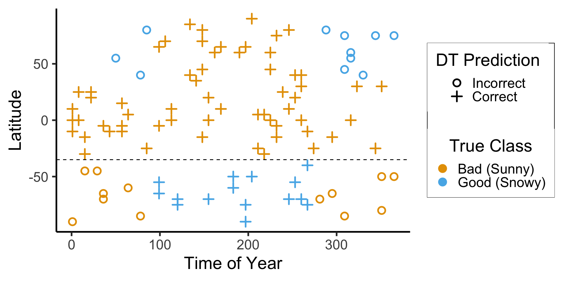
| correct | n |
|---|---|
| FALSE | 24 |
| TRUE | 76 |
\[ \begin{align*} \mathscr{L}(R_1) &= -\left[ \frac{13}{28}\log_2\left(\frac{13}{28}\right) + \frac{15}{28}\log_2\left(\frac{15}{28}\right) \right] \approx 0.996 \\ \mathscr{L}(R_2) &= -\left[ \frac{61}{72}\log_2\left(\frac{61}{72}\right) + \frac{11}{72}\log_2\left(\frac{11}{72}\right) \right] \approx 0.617 \\ %\mathscr{L}(R \rightarrow (R_1, R_2)) &= \Pr(x_i \in R_1)\mathscr{L}(R_1) + \Pr(x_i \in R_2)\mathscr{L}(R_2) \\ \mathscr{L}(R_1, R_2) &= \frac{28}{100}(0.996) + \frac{72}{100}(0.617) \approx 0.723 < 0.827~😻 \end{align*} \]
Continuous Values
- What if we replace binary labels with continuous values: in this case, cm of snow?
Code
#format_snow <- function(x) sprintf('%.2f', x)
format_snow <- function(x) round(x, 2)
ski_sample['snowfall_str'] <- sapply(ski_sample$snowfall, format_snow)
#ski_df |> head()
#print(nrow(ski_df))
ggplot(ski_sample, aes(x=day, y=latitude, label=snowfall_str)) +
  geom_text(size = 6) +
  dsan_theme() +
  labs(
    x = "Time of Year",
    y = "Latitude",
    shape = "Good Skiing?"
  ) +
  scale_shape_manual(values=c(1, 3)) +
  scale_x_continuous(
    breaks=c(ymd('2023-01-01'), ymd('2023-02-01'), ymd('2023-03-01'), ymd('2023-04-01'), ymd('2023-05-01'), ymd('2023-06-01'), ymd('2023-07-01'), ymd('2023-08-01'), ymd('2023-09-01'), ymd('2023-10-01'), ymd('2023-11-01'), ymd('2023-12-01')),
    labels=c("Jan", "Feb", "Mar", "Apr", "May", "Jun", "Jul", "Aug", "Sep", "Oct", "Nov", "Dec")
  ) +
  scale_y_continuous(breaks=c(-90, -60, -30, 0, 30, 60, 90))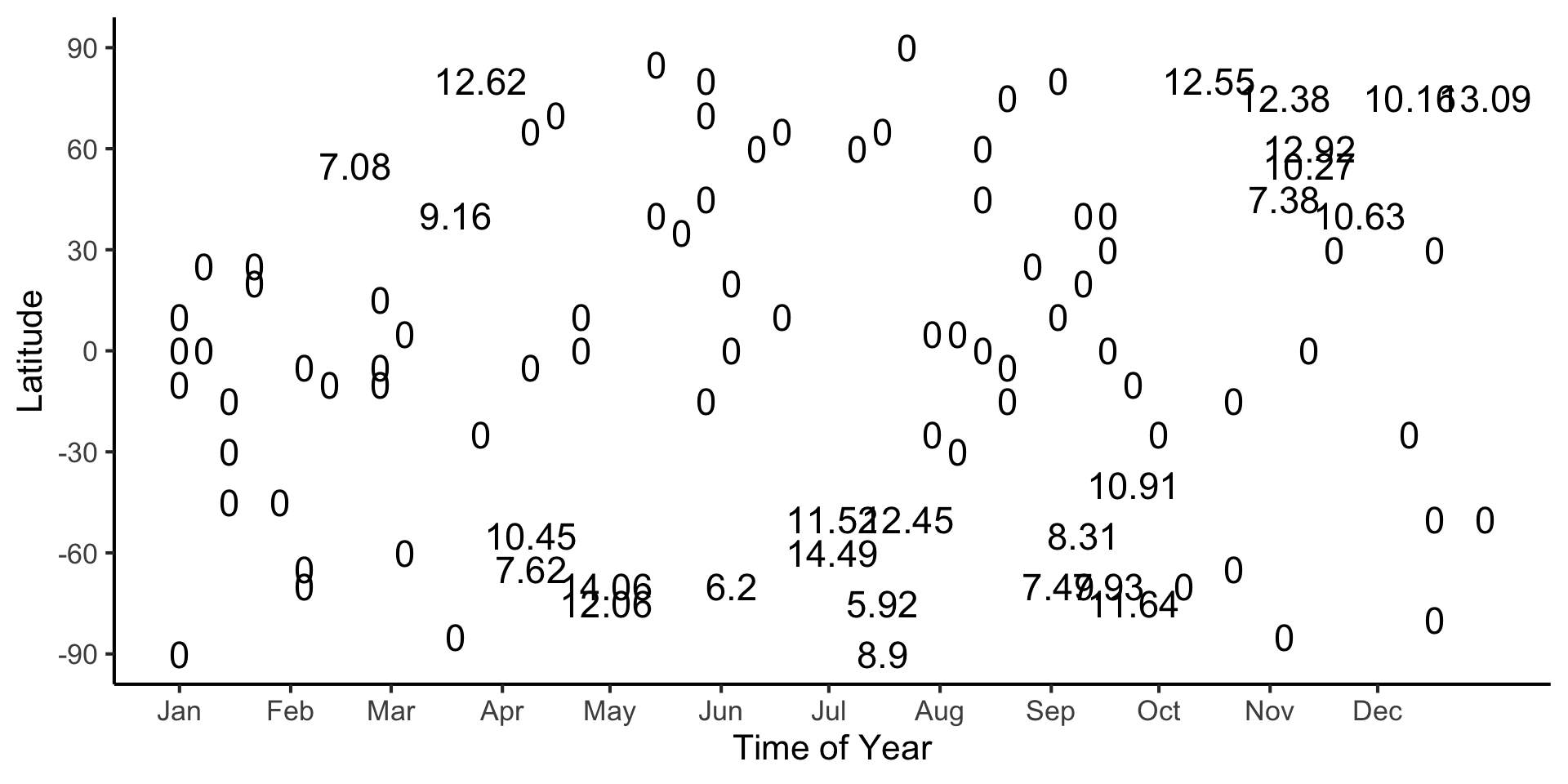
(Example adapted from CS229: Machine Learning, Stanford University)
Looking Towards Regression
- How could we make a decision tree to predict \(y\) from \(x\) for this data?
Code
library(tidyverse)
library(latex2exp)
expr_pi2 <- TeX("$\\frac{\\pi}{2}$")
expr_pi <- TeX("$\\pi$")
expr_3pi2 <- TeX("$\\frac{3\\pi}{2}$")
expr_2pi <- TeX("$2\\pi$")
x_range <- 2 * pi
x_coords <- seq(0, x_range, by = x_range / 100)
num_x_coords <- length(x_coords)
data_df <- tibble(x = x_coords)
data_df <- data_df |> mutate(
  y_raw = sin(x),
  y_noise = rnorm(num_x_coords, 0, 0.15)
)
data_df <- data_df |> mutate(
  y = y_raw + y_noise
)
#y_coords <- y_raw_coords + y_noise
#y_coords <- y_raw_coords
#data_df <- tibble(x = x, y = y)
reg_tree_plot <- ggplot(data_df, aes(x=x, y=y)) +
  geom_point(size = g_pointsize / 2) +
  dsan_theme("half") +
  labs(
    x = "Feature",
    y = "Label"
  ) +
  geom_vline(
    xintercept = pi,
    linewidth = g_linewidth,
    linetype = "dashed"
  ) +
  scale_x_continuous(
    breaks=c(0,pi/2,pi,(3/2)*pi,2*pi),
    labels=c("0",expr_pi2,expr_pi,expr_3pi2,expr_2pi)
  )
reg_tree_plot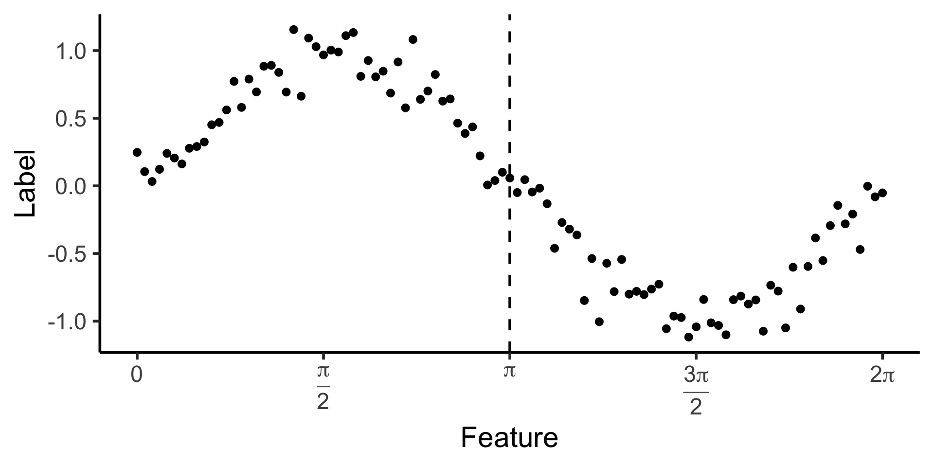
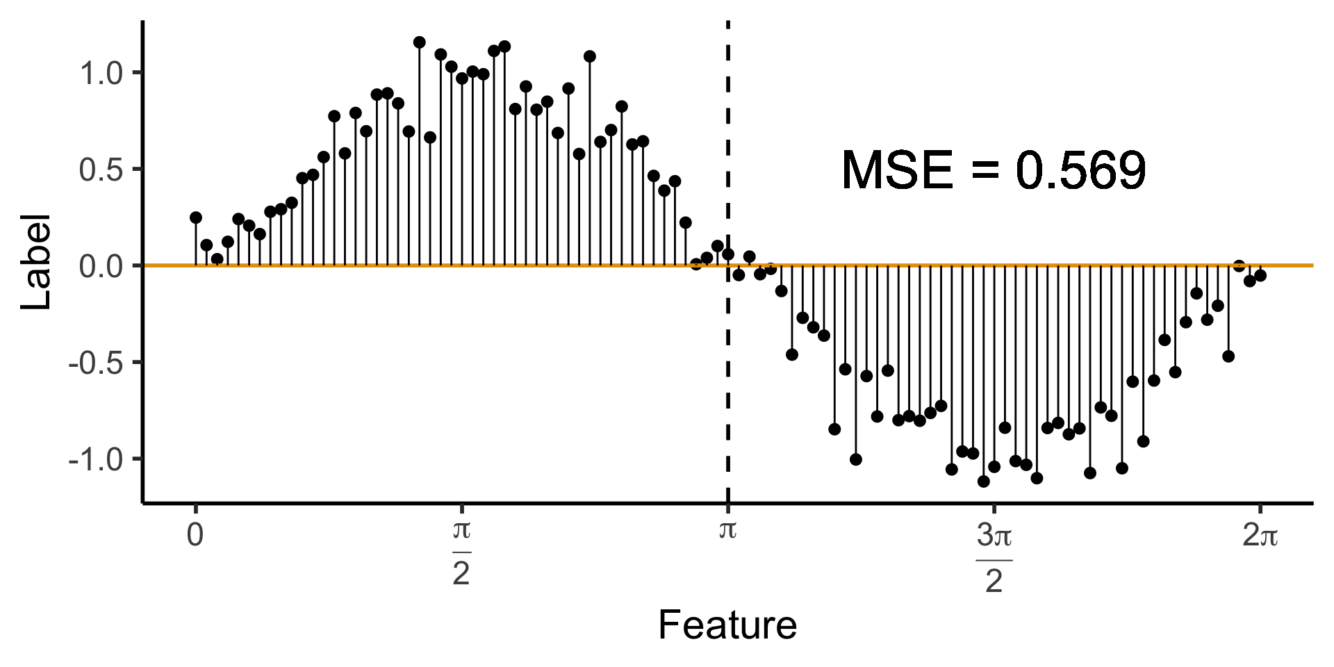
A Zero-Level Tree
- Trivial example: \(\widehat{y}(x) = 0\). How well does this do?
Code
library(ggtext)
# x_lt_pi = data_df |> filter(x < pi)
# mean(x_lt_pi$y)
data_df <- data_df |> mutate(
  pred_sq_err0 = (y - 0)^2
)
mse0 <- mean(data_df$pred_sq_err0)
mse0_str <- sprintf("%.3f", mse0)
reg_tree_plot +
  geom_hline(
    yintercept = 0,
    color=cbPalette[1],
    linewidth = g_linewidth
  ) +
  geom_segment(
    aes(x=x, xend=x, y=0, yend=y)
  ) +
  geom_text(
    aes(x=(3/2)*pi, y=0.5, label=paste0("MSE = ",mse0_str)),
    size = 10,
    #box.padding = unit(c(2,2,2,2), "pt")
  )
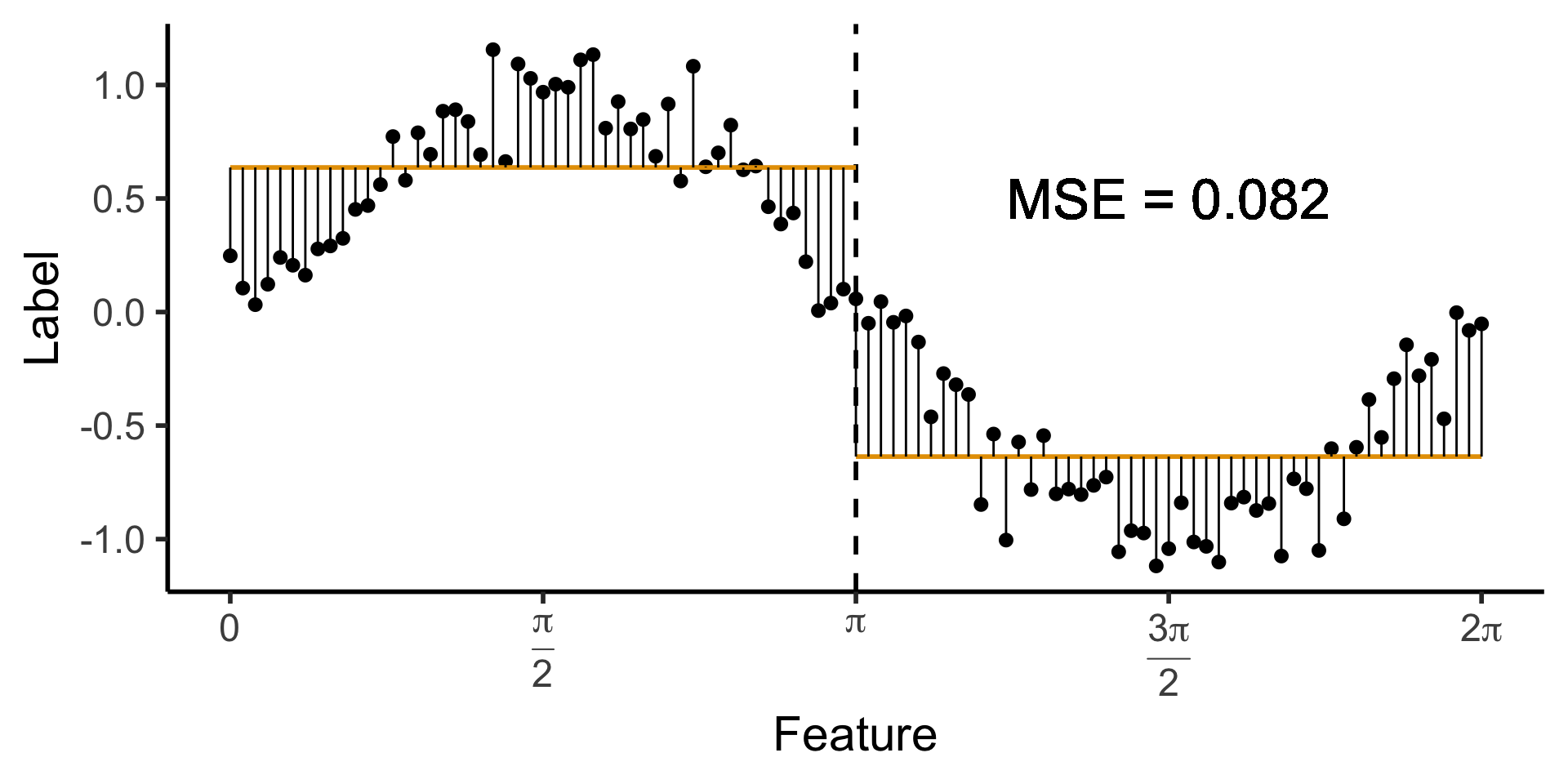
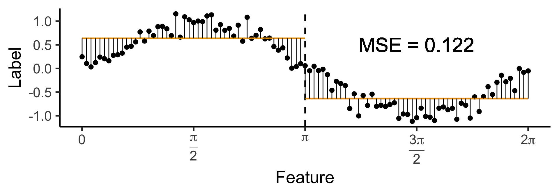
A One-Level Binary Tree
- Let’s introduce a single branch node:
\[ \widehat{y}(x) = \begin{cases} \phantom{-}\frac{2}{\pi} &\text{if }x < \pi, \\ -\frac{2}{\pi} &\text{otherwise.} \end{cases} \]

Code
get_y_pred <- function(x) ifelse(x < pi, 2/pi, -2/pi)
data_df <- data_df |> mutate(
  pred_sq_err1 = (y - get_y_pred(x))^2
)
mse1 <- mean(data_df$pred_sq_err1)
mse1_str <- sprintf("%.3f", mse1)
decision_df <- tribble(
  ~x, ~xend, ~y, ~yend,
  0, pi, 2/pi, 2/pi,
  pi, 2*pi, -2/pi, -2/pi
)
reg_tree_plot +
  geom_segment(
    data=decision_df,
    aes(x=x, xend=xend, y=y, yend=yend),
    color=cbPalette[1],
    linewidth = g_linewidth
  ) +
  geom_segment(
    aes(x=x, xend=x, y=get_y_pred(x), yend=y)
  ) +
  geom_text(
    aes(x=(3/2)*pi, y=0.5, label=paste0("MSE = ",mse1_str)),
    size = 9,
    #box.padding = unit(c(2,2,2,2), "pt")
  )
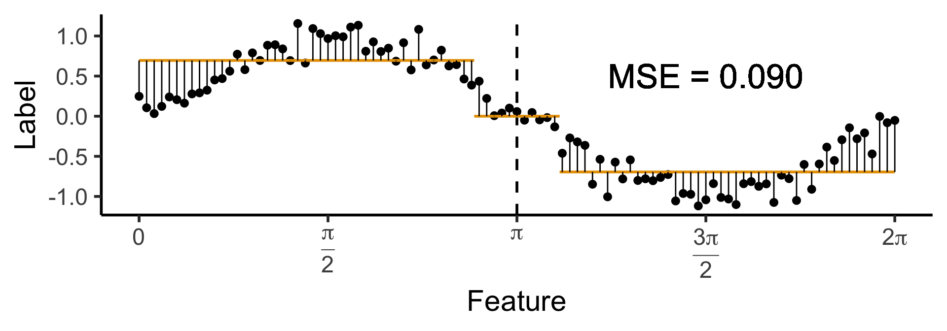
A One-Level Ternary Tree
- Now let’s allow three answers:
\[ \widehat{y}(x) = \begin{cases} \phantom{-}\frac{9}{4\pi} &\text{if }x < \frac{2\pi}{3}, \\ \phantom{-}0 &\text{if }\frac{2\pi}{3} \leq x \leq \frac{4\pi}{3} \\ -\frac{9}{4\pi} &\text{otherwise.} \end{cases} \]

Code
cut1 <- (2/3) * pi
cut2 <- (4/3) * pi
pos_mean <- 9 / (4*pi)
get_y_pred <- function(x) ifelse(x < cut1, pos_mean, ifelse(x < cut2, 0, -pos_mean))
data_df <- data_df |> mutate(
  pred_sq_err1b = (y - get_y_pred(x))^2
)
mse1b <- mean(data_df$pred_sq_err1b)
mse1b_str <- sprintf("%.3f", mse1b)
decision_df <- tribble(
  ~x, ~xend, ~y, ~yend,
  0, (2/3)*pi, pos_mean, pos_mean,
  (2/3)*pi, (4/3)*pi, 0, 0,
  (4/3)*pi, 2*pi, -pos_mean, -pos_mean
)
reg_tree_plot +
  geom_segment(
    data=decision_df,
    aes(x=x, xend=xend, y=y, yend=yend),
    color=cbPalette[1],
    linewidth = g_linewidth
  ) +
  geom_segment(
    aes(x=x, xend=x, y=get_y_pred(x), yend=y)
  ) +
  geom_text(
    aes(x=(3/2)*pi, y=0.5, label=paste0("MSE = ",mse1b_str)),
    size = 9,
    #box.padding = unit(c(2,2,2,2), "pt")
  )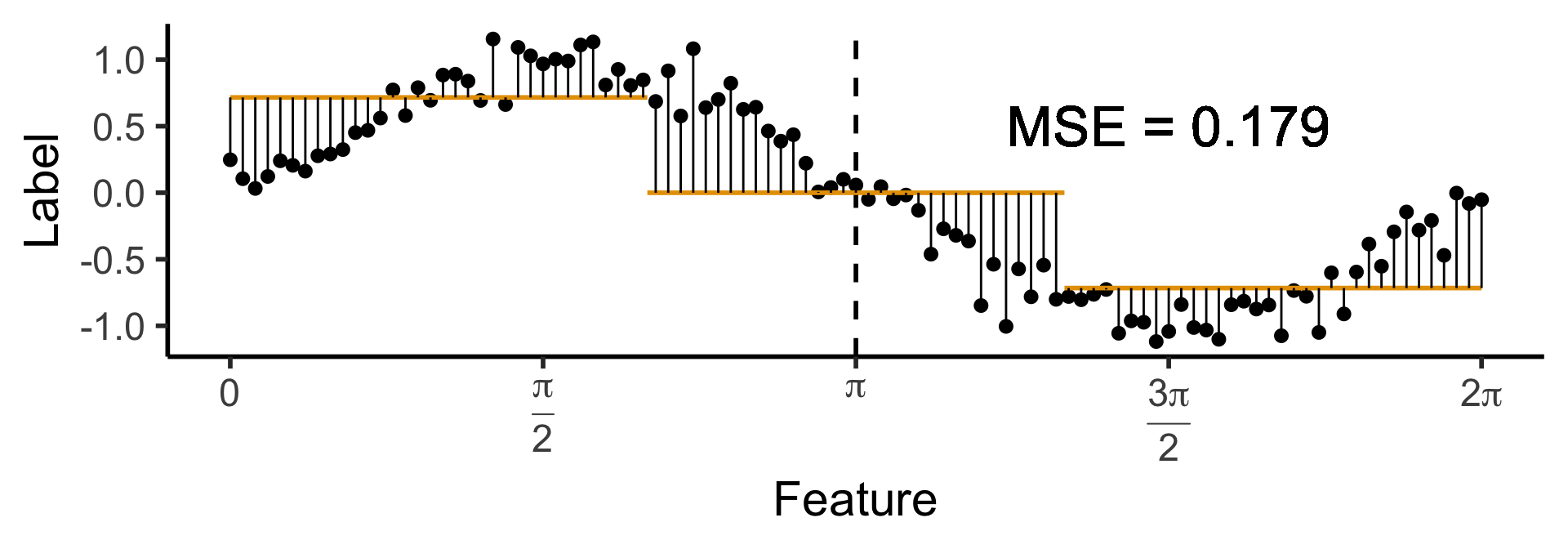
Another One-Level Ternary Tree
- Now let’s allow an uneven split:
\[ \widehat{y}(x) = \begin{cases} \phantom{-}0.695 &\text{if }x < (1-c)\pi, \\ \phantom{-}0 &\text{if }(1-c)\pi \leq x \leq (1+c)\pi \\ -0.695 &\text{otherwise,} \end{cases} \]
with \(c \approx 0.113\), gives us:

Code
c <- 0.113
cut1 <- (1 - c) * pi
cut2 <- (1 + c) * pi
pos_mean <- 0.695
get_y_pred <- function(x) ifelse(x < cut1, pos_mean, ifelse(x < cut2, 0, -pos_mean))
data_df <- data_df |> mutate(
  pred_sq_err1b = (y - get_y_pred(x))^2
)
mse1b <- mean(data_df$pred_sq_err1b)
mse1b_str <- sprintf("%.3f", mse1b)
decision_df <- tribble(
  ~x, ~xend, ~y, ~yend,
  0, cut1, pos_mean, pos_mean,
  cut1, cut2, 0, 0,
  cut2, 2*pi, -pos_mean, -pos_mean
)
reg_tree_plot +
  geom_segment(
    data=decision_df,
    aes(x=x, xend=xend, y=y, yend=yend),
    color=cbPalette[1],
    linewidth = g_linewidth
  ) +
  geom_segment(
    aes(x=x, xend=x, y=get_y_pred(x), yend=y)
  ) +
  geom_text(
    aes(x=(3/2)*pi, y=0.5, label=paste0("MSE = ",mse1b_str)),
    size = 9,
    #box.padding = unit(c(2,2,2,2), "pt")
  )
A Zero-Level Tree
- Trivial example: \(\widehat{y}(x) = 0\). (We ignore the feature value)
- How well does this do?

Code
library(ggtext)
# x_lt_pi = data_df |> filter(x < pi)
# mean(x_lt_pi$y)
data_df <- data_df |> mutate(
  pred_sq_err0 = (y - 0)^2
)
mse0 <- mean(data_df$pred_sq_err0)
mse0_str <- sprintf("%.3f", mse0)
reg_tree_plot +
  geom_hline(
    yintercept = 0,
    color=cbPalette[1],
    linewidth = g_linewidth
  ) +
  geom_segment(
    aes(x=x, xend=x, y=0, yend=y)
  ) +
  geom_text(
    aes(x=(3/2)*pi, y=0.5, label=paste0("MSE = ",mse0_str)),
    size = 10,
    #box.padding = unit(c(2,2,2,2), "pt")
  )
A One-Level Binary Tree
- Let’s introduce a single branch node:
\[ \widehat{y}(x) = \begin{cases} \phantom{-}\frac{2}{\pi} &\text{if }x < \pi, \\ -\frac{2}{\pi} &\text{otherwise.} \end{cases} \]
Code
get_y_pred <- function(x) ifelse(x < pi, 2/pi, -2/pi)
data_df <- data_df |> mutate(
  pred_sq_err1 = (y - get_y_pred(x))^2
)
mse1 <- mean(data_df$pred_sq_err1)
mse1_str <- sprintf("%.3f", mse1)
decision_df <- tribble(
  ~x, ~xend, ~y, ~yend,
  0, pi, 2/pi, 2/pi,
  pi, 2*pi, -2/pi, -2/pi
)
reg_tree_plot +
  geom_segment(
    data=decision_df,
    aes(x=x, xend=xend, y=y, yend=yend),
    color=cbPalette[1],
    linewidth = g_linewidth
  ) +
  geom_segment(
    aes(x=x, xend=x, y=get_y_pred(x), yend=y)
  ) +
  geom_text(
    aes(x=(3/2)*pi, y=0.5, label=paste0("MSE = ",mse1_str)),
    size = 9,
    #box.padding = unit(c(2,2,2,2), "pt")
  )
A One-Level Ternary Tree
- Now let’s allow three answers:
\[ \widehat{y}(x) = \begin{cases} \phantom{-}\frac{9}{4\pi} &\text{if }x < \frac{2\pi}{3}, \\ \phantom{-}0 &\text{if }\frac{2\pi}{3} \leq x \leq \frac{4\pi}{3} \\ -\frac{9}{4\pi} &\text{otherwise.} \end{cases} \]
Code
cut1 <- (2/3) * pi
cut2 <- (4/3) * pi
pos_mean <- 9 / (4*pi)
get_y_pred <- function(x) ifelse(x < cut1, pos_mean, ifelse(x < cut2, 0, -pos_mean))
data_df <- data_df |> mutate(
  pred_sq_err1b = (y - get_y_pred(x))^2
)
mse1b <- mean(data_df$pred_sq_err1b)
mse1b_str <- sprintf("%.3f", mse1b)
decision_df <- tribble(
  ~x, ~xend, ~y, ~yend,
  0, (2/3)*pi, pos_mean, pos_mean,
  (2/3)*pi, (4/3)*pi, 0, 0,
  (4/3)*pi, 2*pi, -pos_mean, -pos_mean
)
reg_tree_plot +
  geom_segment(
    data=decision_df,
    aes(x=x, xend=xend, y=y, yend=yend),
    color=cbPalette[1],
    linewidth = g_linewidth
  ) +
  geom_segment(
    aes(x=x, xend=x, y=get_y_pred(x), yend=y)
  ) +
  geom_text(
    aes(x=(3/2)*pi, y=0.5, label=paste0("MSE = ",mse1b_str)),
    size = 9,
    #box.padding = unit(c(2,2,2,2), "pt")
  )
Another One-Level Ternary Tree
- Now let’s allow an uneven split:
\[ \widehat{y}(x) = \begin{cases} \phantom{-}0.695 &\text{if }x < (1-c)\pi, \\ \phantom{-}0 &\text{if }(1-c)\pi \leq x \leq (1+c)\pi \\ -0.695 &\text{otherwise,} \end{cases} \]
with \(c \approx 0.113\), gives us:
Code
c <- 0.113
cut1 <- (1 - c) * pi
cut2 <- (1 + c) * pi
pos_mean <- 0.695
get_y_pred <- function(x) ifelse(x < cut1, pos_mean, ifelse(x < cut2, 0, -pos_mean))
data_df <- data_df |> mutate(
  pred_sq_err1b = (y - get_y_pred(x))^2
)
mse1b <- mean(data_df$pred_sq_err1b)
mse1b_str <- sprintf("%.3f", mse1b)
decision_df <- tribble(
  ~x, ~xend, ~y, ~yend,
  0, cut1, pos_mean, pos_mean,
  cut1, cut2, 0, 0,
  cut2, 2*pi, -pos_mean, -pos_mean
)
reg_tree_plot +
  geom_segment(
    data=decision_df,
    aes(x=x, xend=xend, y=y, yend=yend),
    color=cbPalette[1],
    linewidth = g_linewidth
  ) +
  geom_segment(
    aes(x=x, xend=x, y=get_y_pred(x), yend=y)
  ) +
  geom_text(
    aes(x=(3/2)*pi, y=0.5, label=paste0("MSE = ",mse1b_str)),
    size = 9,
    #box.padding = unit(c(2,2,2,2), "pt")
  )
Getting Closer
- Your first instinct might be to choose the misclassification rate, the proportion of points in region \(R\) that we are misclassifying if we guess the most-common class:
\[ \mathscr{L}_{MC}(R) = 1 - \widehat{p}_{R} \]
- The shape of this function, however, gives us a hint as to why we may want to choose a different function:
Code
library(tidyverse)
library(latex2exp)
my_mc <- function(p) 0.5 - abs(0.5 - p)
x_vals <- seq(0, 1, 0.01)
mc_vals <- sapply(x_vals, my_mc)
phat_label <- TeX('$\\widehat{p}$')
data_df <- tibble(x=x_vals, loss_mc=mc_vals)
ggplot(data_df, aes(x=x, y=loss_mc)) +
  geom_line(linewidth = g_linewidth) +
  dsan_theme("half") +
  labs(
    x = phat_label,
    y = "Misclassification Loss"
  )
Using Misclassification Loss to Choose a Split
- Given a parent region \(R_P\), we’re trying to choose a split into subregions \(R_1\) and \(R_2\) which will decrease the loss: \(\frac{|R_1|}{|R_P|}\mathscr{L}(R_1) + \frac{|R_2|}{|R_P|}\mathscr{L}(R_2) < \mathscr{L}(R_P)\)
- But what happens when we use misclassification loss to “judge” a split?

- Tl;dr this doesn’t “detect” when we’ve reduced uncertainty
- But we do have a function that was constructed to measure uncertainty!
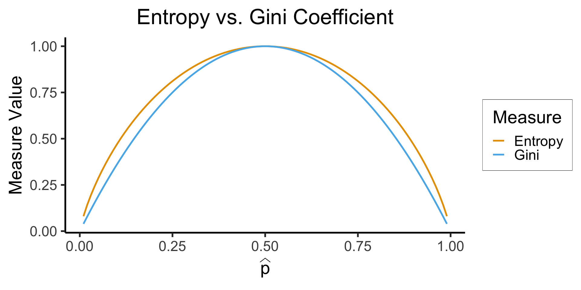
Using Entropy to Choose a Split

Is There Another Option?
\[ \mathscr{L}_{\text{Ent}}(\widehat{p}) = -\sum_{i=1}^K \widehat{p}_k\log_2(\widehat{p}_k) \]
\[ \mathscr{L}_{\text{Gini}}(\widehat{p}) = -\sum_{i=1}^K \widehat{p}_k(1-\widehat{p}_k) \]
Code
library(tidyverse)
library(latex2exp)
phat_label <- TeX('$\\widehat{p}')
my_ent <- function(p) -(p*log2(p) + (1-p)*log2(1-p))
my_gini <- function(p) 4*p*(1-p)
x_vals <- seq(0.01, 0.99, 0.01)
ent_vals <- sapply(x_vals, my_ent)
ent_df <- tibble(x=x_vals, y=ent_vals, Measure="Entropy")
gini_vals <- sapply(x_vals, my_gini)
gini_df <- tibble(x=x_vals, y=gini_vals, Measure="Gini")
data_df <- bind_rows(ent_df, gini_df)
ggplot(data=data_df, aes(x=x, y=y, color=Measure)) +
  geom_line(linewidth = g_linewidth) +
  dsan_theme("half") +
  scale_color_manual(values=c(cbPalette[1], cbPalette[2])) +
  labs(
    x = phat_label,
    y = "Measure Value",
    title = "Entropy vs. Gini Coefficient"
  )
The Space of All Decision Trees
- Why can’t we just try all possible decision trees, and choose the one with minimum loss? Consider a case with just \(N = 1\) binary feature, \(F_1 \in \{0, 1\}\):


Back to the Skiing Example
Code
library(tidyverse)
library(lubridate)
set.seed(5001)
sample_size <- 100
day <- seq(ymd('2023-01-01'),ymd('2023-12-31'),by='weeks')
lat_bw <- 5
latitude <- seq(-90, 90, by=lat_bw)
ski_df <- expand_grid(day, latitude)
ski_df <- tibble::rowid_to_column(ski_df, var='obs_id')
#ski_df |> head()
# Data-generating process
lat_cutoff <- 35
ski_df <- ski_df |> mutate(
  near_equator = abs(latitude) <= lat_cutoff,
  northern = latitude > lat_cutoff,
  southern = latitude < -lat_cutoff,
  first_3m = day < ymd('2023-04-01'),
  last_3m = day >= ymd('2023-10-01'),
  middle_6m = (day >= ymd('2023-04-01')) & (day < ymd('2023-10-01')),
  snowfall = 0
)
# Update the non-zero sections
mu_snow <- 10
sd_snow <- 2.5
# How many northern + first 3 months
num_north_first_3 <- nrow(ski_df[ski_df$northern & ski_df$first_3m,])
ski_df[ski_df$northern & ski_df$first_3m, 'snowfall'] = rnorm(num_north_first_3, mu_snow, sd_snow)
# Northerns + last 3 months
num_north_last_3 <- nrow(ski_df[ski_df$northern & ski_df$last_3m,])
ski_df[ski_df$northern & ski_df$last_3m, 'snowfall'] = rnorm(num_north_last_3, mu_snow, sd_snow)
# How many southern + middle 6 months
num_south_mid_6 <- nrow(ski_df[ski_df$southern & ski_df$middle_6m,])
ski_df[ski_df$southern & ski_df$middle_6m, 'snowfall'] = rnorm(num_south_mid_6, mu_snow, sd_snow)
# And collapse into binary var
ski_df['good_skiing'] = ski_df$snowfall > 0
# This converts day into an int
ski_df <- ski_df |> mutate(
  day_num = lubridate::yday(day)
)
#print(nrow(ski_df))
ski_sample <- ski_df |> slice_sample(n = sample_size)
ski_sample |> write_csv("assets/ski.csv")
month_vec <- c(ymd('2023-01-01'), ymd('2023-02-01'), ymd('2023-03-01'), ymd('2023-04-01'), ymd('2023-05-01'), ymd('2023-06-01'), ymd('2023-07-01'), ymd('2023-08-01'), ymd('2023-09-01'), ymd('2023-10-01'), ymd('2023-11-01'), ymd('2023-12-01'))
month_labels <- c("Jan", "Feb", "Mar", "Apr", "May", "Jun", "Jul", "Aug", "Sep", "Oct", "Nov", "Dec")
lat_vec <- c(-90, -60, -30, 0, 30, 60, 90)
ggplot(
  ski_sample,
  aes(
    x=day,
    y=latitude,
    #shape=good_skiing,
    color=good_skiing
  )) +
  geom_point(
    size = g_pointsize / 1.5,
    #stroke=1.5
  ) +
  dsan_theme() +
  labs(
    x = "Time of Year",
    y = "Latitude",
    shape = "Good Skiing?"
  ) +
  scale_shape_manual(name="Good Skiing?", values=c(1, 3)) +
  scale_color_manual(name="Good Skiing?", values=c(cbPalette[1], cbPalette[2]), labels=c("No (Sunny)","Yes (Snowy)")) +
  scale_x_continuous(
    breaks=c(month_vec,ymd('2024-01-01')),
    labels=c(month_labels,"Jan")
  ) +
  scale_y_continuous(breaks=lat_vec)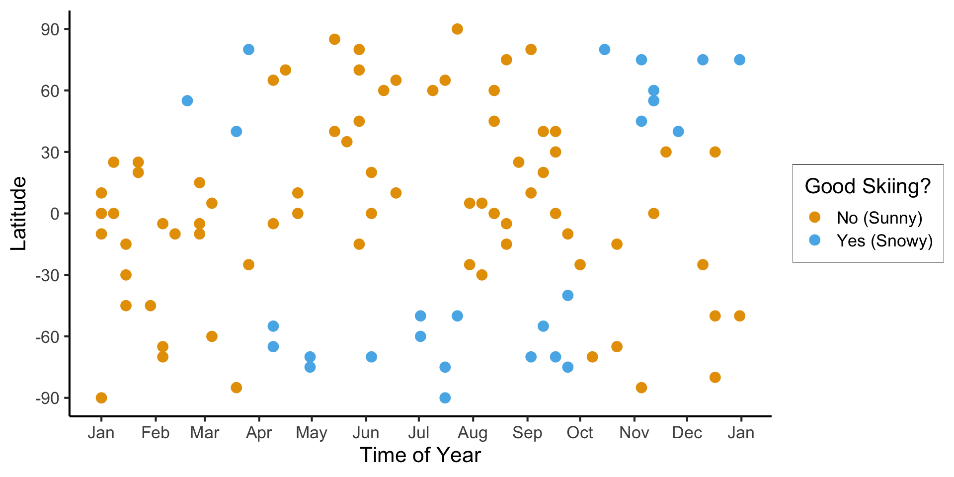
(Example adapted from CS229: Machine Learning, Stanford University)
Your Opponents

High Variance, Low Bias

The Wisdom of Sheep
- Unfortunately, the “wisdom of crowds” phenomenon only works if everyone in the crowd is unable to communicate
- The minute people tasked with making decisions as a group begin to communicate (long story short), they begin to follow charismatic leaders
![]() , and the effect goes away (biases no longer cancel out)
, and the effect goes away (biases no longer cancel out) - The takeaway for effectively training random forests: ensure that each tree has a separate (ideally orthogonal) slice of the full dataset, and has to infer labels from only that slice!
Decision Trees: What Now?
- We have a dataset and a decision tree… now what?
- If our only goal is interpretability, we’re done
- If we want to increase accuracy/efficiency, however, we can do better!

Bootstrapped Trees

Boosting
- Rather than giving each subtree a random subset of features, grow trees sequentially! Ask each subtree to explain remaining unexplained variance from previous step
- Step 1: \(\widehat{f}_1(X)\) = DT for \(X \rightarrow Y\)
- Step \(t+1\): \(\widehat{f}_{t+1}(X)\) = DT for \(X \rightarrow \left(\widehat{f}_t(X) - Y\right)\)
Code
library(ggtext)
# x_lt_pi = data_df |> filter(x < pi)
# mean(x_lt_pi$y)
data_df <- data_df |> mutate(
  pred_sq_err0 = (y - 0)^2
)
mse0 <- mean(data_df$pred_sq_err0)
mse0_str <- sprintf("%.3f", mse0)
reg_tree_plot +
  geom_hline(
    yintercept = 0,
    color=cbPalette[1],
    linewidth = g_linewidth
  ) +
  geom_segment(
    aes(x=x, xend=x, y=0, yend=y)
  ) +
  geom_text(
    aes(x=(3/2)*pi, y=0.5, label=paste0("MSE = ",mse0_str)),
    size = 10,
    #box.padding = unit(c(2,2,2,2), "pt")
  )
get_y_pred <- function(x) ifelse(x < pi, 2/pi, -2/pi)
data_df <- data_df |> mutate(
  pred_sq_err1 = (y - get_y_pred(x))^2
)
mse1 <- mean(data_df$pred_sq_err1)
mse1_str <- sprintf("%.3f", mse1)
decision_df <- tribble(
  ~x, ~xend, ~y, ~yend,
  0, pi, 2/pi, 2/pi,
  pi, 2*pi, -2/pi, -2/pi
)
reg_tree_plot +
  geom_segment(
    data=decision_df,
    aes(x=x, xend=xend, y=y, yend=yend),
    color=cbPalette[1],
    linewidth = g_linewidth
  ) +
  geom_segment(
    aes(x=x, xend=x, y=get_y_pred(x), yend=y)
  ) +
  geom_text(
    aes(x=(3/2)*pi, y=0.5, label=paste0("MSE = ",mse1_str)),
    size = 9,
    #box.padding = unit(c(2,2,2,2), "pt")
)- Original data
- One-level DT