Week 10: Decision Trees

DSAN 5000: Data Science and Analytics

Class Sessions

Author

Prof. Jeff and Prof. James

Published

Thursday, November 7, 2024

Open slides in new window →

Week 9 Recap

Reducing Dimensionality

Method 1: Feature Selection. Selecting a subset of existing features:

\(F_1\)	\(F_2\)	\(F_3\)
0.8	0.9	0.1
0.6	0.4	0.1

→

\(F_1\)	\(F_2\)	\(F_3\)
0.8	0.9	0.1
0.6	0.4	0.1

→

\(F_1\)	\(F_3\)
0.8	0.1
0.6	0.1

Method 2: Feature Extraction. Constructing new features as combinations/functions of the original features

\(F_1\)	\(F_2\)	\(F_3\)
0.8	0.9	0.1
0.6	0.4	0.1

→

\[ \begin{align*} {\color{#56b4e9}F'_{12}} &= \frac{{\color{#e69f00}F_1} + {\color{#e69f00}F_2}}{2} \\ {\color{#56b4e9}F'_{23}} &= \frac{{\color{#e69f00}F_2} + {\color{#e69f00}F_3}}{2} \end{align*} \]

→

\(F'_{12}\)	\(F'_{23}\)
0.85	0.50
0.50	0.25

Principal Component Analysis (PCA)

We know this is feature extraction since we obtain new dimensions:

Code

library(readr)
library(ggplot2)
gdp_df <- read_csv("assets/gdp_pca.csv")

dist_to_line <- function(x0, y0, a, c) {
    numer <- abs(a * x0 - y0 + c)
    denom <- sqrt(a * a + 1)
    return(numer / denom)
}
# Finding PCA line for industrial vs. exports
x <- gdp_df$industrial
y <- gdp_df$exports
lossFn <- function(lineParams, x0, y0) {
    a <- lineParams[1]
    c <- lineParams[2]
    return(sum(dist_to_line(x0, y0, a, c)))
}
o <- optim(c(0, 0), lossFn, x0 = x, y0 = y)
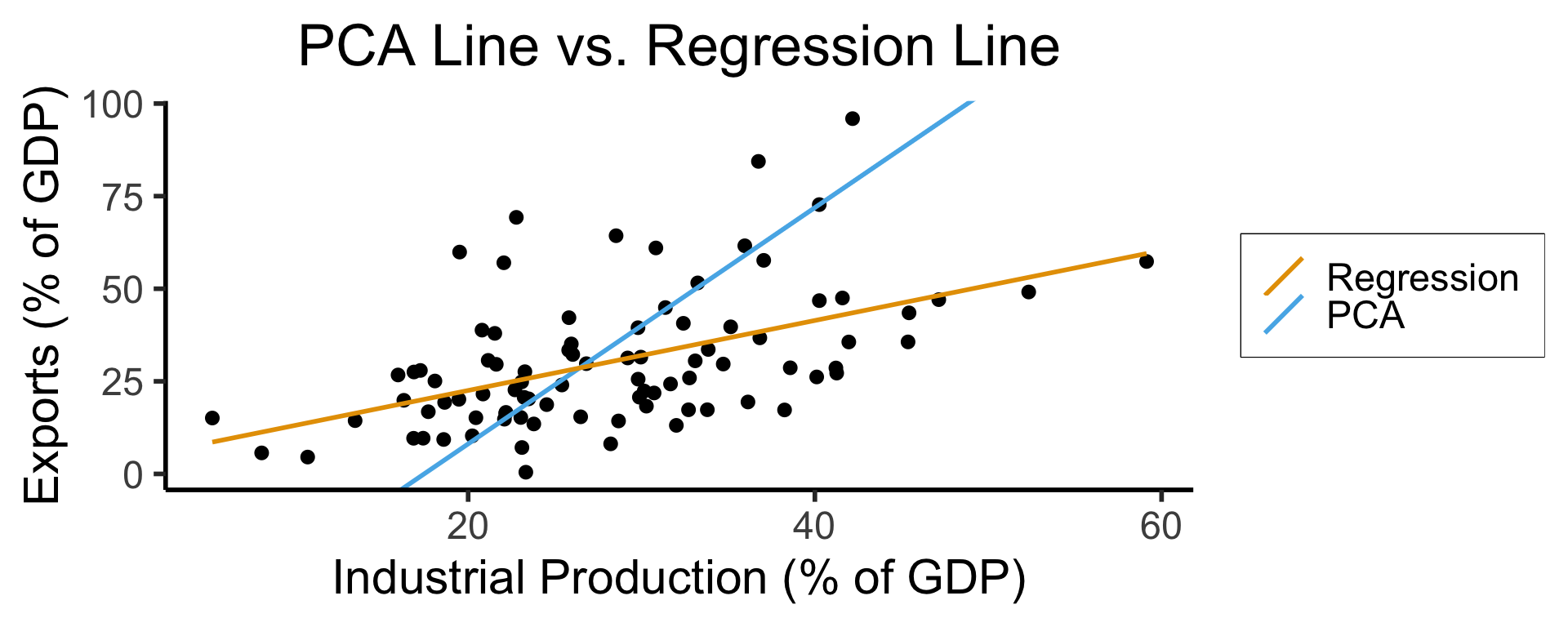
ggplot(gdp_df, aes(x = industrial, y = exports)) +
    geom_point(size=g_pointsize/2) +
    geom_abline(aes(slope = o$par[1], intercept = o$par[2], color="pca"), linewidth=g_linewidth, show.legend = TRUE) +
    geom_smooth(aes(color="lm"), method = "lm", se = FALSE, linewidth=g_linewidth, key_glyph = "blank") +
    scale_color_manual(element_blank(), values=c("pca"=cbPalette[2],"lm"=cbPalette[1]), labels=c("Regression","PCA")) +
    dsan_theme("half") +
    remove_legend_title() +
    labs(
      title = "PCA Line vs. Regression Line",
        x = "Industrial Production (% of GDP)",
        y = "Exports (% of GDP)"
    )
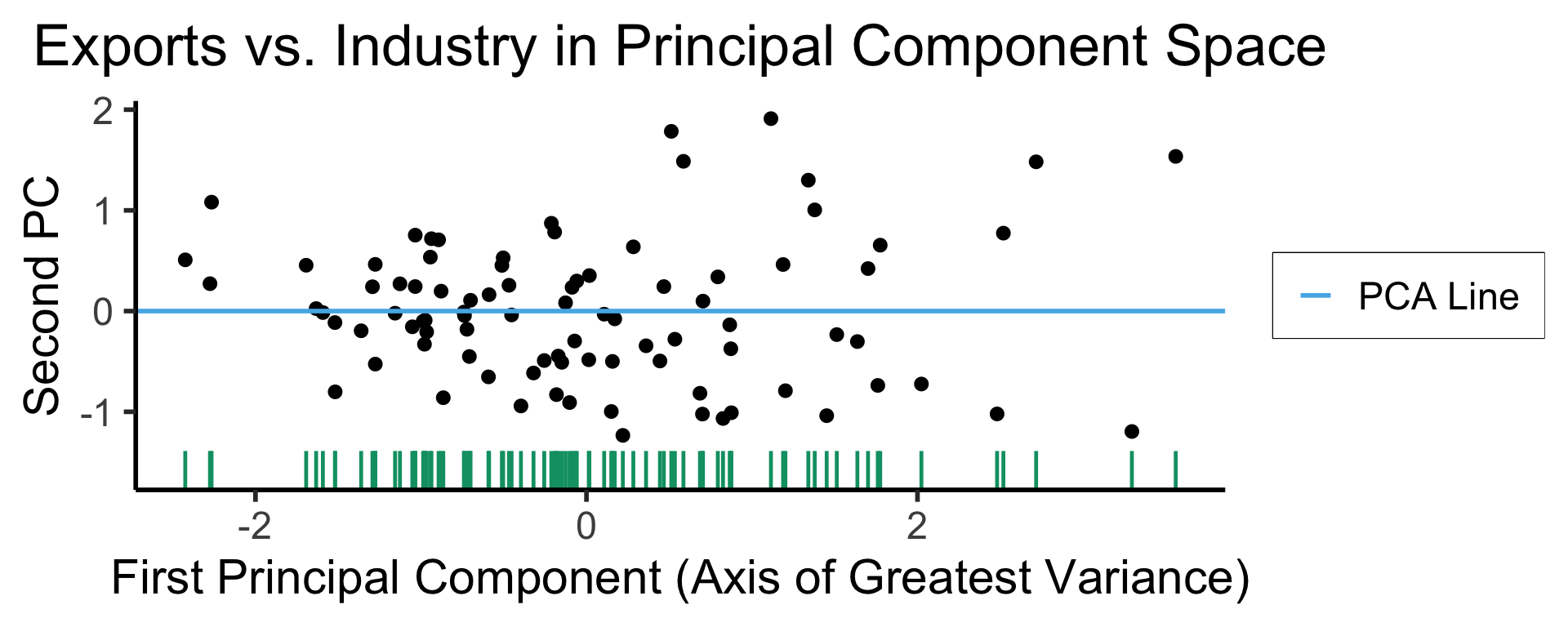
ggplot(gdp_df, aes(pc1, .fittedPC2)) +
    geom_point(size = g_pointsize/2) +
    geom_hline(aes(yintercept=0, color='PCA Line'), linetype='solid', size=g_linesize) +
    geom_rug(sides = "b", linewidth=g_linewidth/1.2, length = unit(0.1, "npc"), color=cbPalette[3]) +
    expand_limits(y=-1.6) +
    scale_color_manual(element_blank(), values=c("PCA Line"=cbPalette[2])) +
    dsan_theme("half") +
    remove_legend_title() +
    labs(
      title = "Exports vs. Industry in Principal Component Space",
      x = "First Principal Component (Axis of Greatest Variance)",
      y = "Second PC"
    )

Code

library(dplyr)
library(tidyr)
plot_df <- gdp_df %>% select(c(country_code, pc1, agriculture, military))
long_df <- plot_df %>% pivot_longer(!c(country_code, pc1), names_to = "var", values_to = "val")
long_df <- long_df |> mutate(
  var = case_match(
    var,
    "agriculture" ~ "Agricultural Production",
    "military" ~ "Military Spending"
  )
)
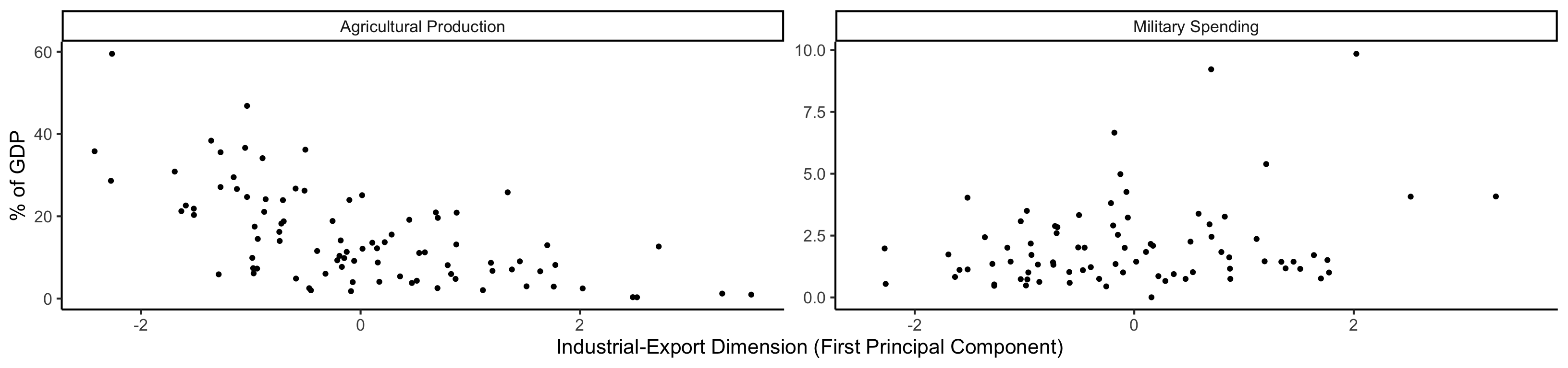
ggplot(long_df, aes(x = pc1, y = val, facet = var)) +
    geom_point() +
    facet_wrap(vars(var), scales = "free") +
    dsan_theme("full") +
    labs(
        x = "Industrial-Export Dimension (First Principal Component)",
        y = "% of GDP"
    )

PCA Math Magic

Remember that our goal is to find the axes along which the data has greatest variance (out of all possible axes)
Let’s create a dataset using a known data-generating process: one dimension with 75% of the total variance, and the second with 25%:

Code

library(tidyverse)
library(MASS)
library(ggforce)
N <- 300
Mu <- c(0, 0)
var_x <- 3
var_y <- 1
Sigma <- matrix(c(var_x, 0, 0, var_y), nrow=2)
data_df <- as_tibble(mvrnorm(N, Mu, Sigma, empirical=TRUE))
colnames(data_df) <- c("x","y")
# data_df <- data_df |> mutate(
#   within_5 = x < 5,
#   within_sq5 = x < sqrt(5)
# )
#nrow(data_df |> filter(within_5)) / nrow(data_df)
#nrow(data_df |> filter(within_sq5)) / nrow(data_df)
# And plot
ggplot(data_df, aes(x=x, y=y)) +
  # 68% ellipse
  # stat_ellipse(geom="polygon", type="norm", linewidth=g_linewidth, level=0.68, fill=cbPalette[1], alpha=0.5) +
  # stat_ellipse(type="norm", linewidth=g_linewidth, level=0.68) +
  geom_ellipse(
    aes(x0=0, y0=0, a=var_x, b=var_y, angle=0),
    linewidth = g_linewidth
  ) +
  # geom_ellipse(
  #   aes(x0=0, y0=0, a=sqrt(5), b=1, angle=0),
  #   linewidth = g_linewidth,
  #   geom="polygon",
  #   fill=cbPalette[1], alpha=0.2
  # ) +
  # # 95% ellipse
  # stat_ellipse(geom="polygon", type="norm", linewidth=g_linewidth, level=0.95, fill=cbPalette[1], alpha=0.25) +
  # stat_ellipse(type="norm", linewidth=g_linewidth, level=0.95) +
  # # 99.7% ellipse
  # stat_ellipse(geom='polygon', type="norm", linewidth=g_linewidth, level=0.997, fill=cbPalette[1], alpha=0.125) +
  # stat_ellipse(type="norm", linewidth=g_linewidth, level=0.997) +
  # Lines at x=0 and y=0
  geom_vline(xintercept=0, linetype="dashed", linewidth=g_linewidth / 2) +
  geom_hline(yintercept=0, linetype="dashed", linewidth = g_linewidth / 2) +
  geom_point(
    size = g_pointsize / 3,
    #alpha=0.5
  ) +
  geom_rug(length=unit(0.5, "cm"), alpha=0.75) +
  geom_segment(
    aes(x=-var_x, y=0, xend=var_x, yend=0, color='PC1'),
    linewidth = 1.5 * g_linewidth,
    arrow = arrow(length = unit(0.1, "npc"))
  ) +
  geom_segment(
    aes(x=0, y=-var_y, xend=0, yend=var_y, color='PC2'),
    linewidth = 1.5 * g_linewidth,
    arrow = arrow(length = unit(0.1, "npc"))
  ) +
  dsan_theme("half") +
  coord_fixed() +
  remove_legend_title() +
  scale_color_manual(
    "PC Vectors",
    values=c('PC1'=cbPalette[1], 'PC2'=cbPalette[2])
  ) +
  scale_x_continuous(breaks=seq(-5,5,1), limits=c(-5,5))

── Attaching core tidyverse packages ──────────────────────── tidyverse 2.0.0 ──
✔ forcats   1.0.0     ✔ stringr   1.5.1
✔ lubridate 1.9.3     ✔ tibble    3.2.1
✔ purrr     1.0.2     
── Conflicts ────────────────────────────────────────── tidyverse_conflicts() ──
✖ dplyr::filter() masks stats::filter()
✖ dplyr::lag()    masks stats::lag()
ℹ Use the conflicted package (<http://conflicted.r-lib.org/>) to force all conflicts to become errors


Attaching package: 'MASS'

The following object is masked from 'package:dplyr':

    select

Warning: The `x` argument of `as_tibble.matrix()` must have unique column names if
`.name_repair` is omitted as of tibble 2.0.0.
ℹ Using compatibility `.name_repair`.

Warning in geom_segment(aes(x = -var_x, y = 0, xend = var_x, yend = 0, color = "PC1"), : All aesthetics have length 1, but the data has 300 rows.
ℹ Please consider using `annotate()` or provide this layer with data containing
  a single row.

Warning in geom_segment(aes(x = 0, y = -var_y, xend = 0, yend = var_y, color = "PC2"), : All aesthetics have length 1, but the data has 300 rows.
ℹ Please consider using `annotate()` or provide this layer with data containing
  a single row.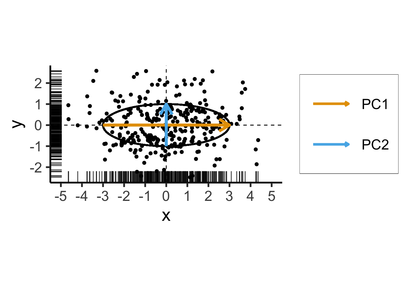

\[ \mathbf{\Sigma} = \begin{bmatrix} {\color{#e69f00}3} & 0 \\ 0 & {\color{#56b4e9}1} \end{bmatrix} \]

Two solutions to \(\mathbf{\Sigma}\mathbf{x} = \lambda \mathbf{x}\):

\({\color{#e69f00}\lambda_1} = 3, {\color{#e69f00}\mathbf{x}_1} = (1, 0)^\top\)
\({\color{#56b4e9}\lambda_2} = 1, {\color{#56b4e9}\mathbf{x}_2} = (0, 1)^\top\)

Now With PCA Lines \(\neq\) Axes

We now introduce covariance between \(x\) and \(y\) coordinates of our data:

Code

library(tidyverse)
library(MASS)
N <- 250
Mu <- c(0,0)
Sigma <- matrix(c(2,1,1,2), nrow=2)
data_df <- as_tibble(mvrnorm(N, Mu, Sigma))
colnames(data_df) <- c("x","y")
# Start+end coordinates for the transformed vectors
pc1_rc <- (3/2)*sqrt(2)
pc2_rc <- (1/2)*sqrt(2)
ggplot(data_df, aes(x=x, y=y)) +
  geom_ellipse(
    aes(x0=0, y0=0, a=var_x, b=var_y, angle=pi/4),
    linewidth = g_linewidth,
    #fill='grey', alpha=0.0075
  ) +
  geom_vline(xintercept=0, linetype="dashed", linewidth=g_linewidth / 2) +
  geom_hline(yintercept=0, linetype="dashed", linewidth = g_linewidth / 2) +
  geom_point(
    size = g_pointsize / 3,
    #alpha=0.7
  ) +
  geom_rug(
    length=unit(0.35, "cm"), alpha=0.75
  ) +
  geom_segment(
    aes(x=-pc1_rc, y=-pc1_rc, xend=pc1_rc, yend=pc1_rc, color='PC1'),
    linewidth = 1.5 * g_linewidth,
    arrow = arrow(length = unit(0.1, "npc"))
  ) +
  geom_segment(
    aes(x=pc2_rc, y=-pc2_rc, xend=-pc2_rc, yend=pc2_rc, color='PC2'),
    linewidth = 1.5 * g_linewidth,
    arrow = arrow(length = unit(0.1, "npc"))
  ) +
  dsan_theme("half") +
  remove_legend_title() +
  coord_fixed() +
  scale_x_continuous(breaks=seq(-4,4,2))

Warning in geom_segment(aes(x = -pc1_rc, y = -pc1_rc, xend = pc1_rc, yend = pc1_rc, : All aesthetics have length 1, but the data has 250 rows.
ℹ Please consider using `annotate()` or provide this layer with data containing
  a single row.

Warning in geom_segment(aes(x = pc2_rc, y = -pc2_rc, xend = -pc2_rc, yend = pc2_rc, : All aesthetics have length 1, but the data has 250 rows.
ℹ Please consider using `annotate()` or provide this layer with data containing
  a single row.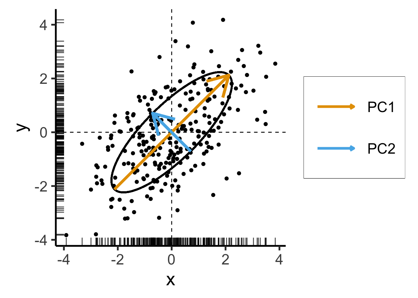

\[ \mathbf{\Sigma}' = \begin{bmatrix} 2 & 1 \\ 1 & 2 \end{bmatrix} \]

Still two solutions to \(\mathbf{\Sigma}'\mathbf{x} = \lambda \mathbf{x}\):

\({\color{#e69f00}\lambda_1} = 3, {\color{#e69f00}\mathbf{x}_1} = (1,1)^\top\)
\({\color{#56b4e9}\lambda_2} = 1, {\color{#56b4e9}\mathbf{x}_2} = (-1,1)^\top\)

For those interested in how we obtained \(\mathbf{\Sigma}'\) with same eigenvalues but different eigenvectors from \(\mathbf{\Sigma}\), see the appendix slide.

PCA and Eigenvalues

Takeaway 1: Regardless of the coordinate system,

Eigenvectors give us axes of greatest variance: \(\mathbf{x}_1\) is axis of greatest variance, \(\mathbf{x}_2\) is axis of 2nd-greatest variance, etc.
The corresponding Eigenvalues tell us how much of the total variance is explained by this axis

PCA as Swiss Army Knife

PCA can be used for both reinterpretation and reduction of dimensions!
Consider dataset \(\mathbf{X} = (X_1, \ldots, X_n)\), with \(X_i \in \mathbb{R}^N\)

Reinterpretation

If we project each \(X_i\) onto \(N\) principal component axes:

Datapoints in PC space are linear combinations of the original datapoints! (← Takeaway 2a)

\[ X'_i = \alpha_1X_1 + \cdots + \alpha_nX_n, \]

where \(\forall i \left[\alpha_i \neq 0\right]\)
We are just “re-plotting” our original data in PC space via change of coordinates
Thus we can recover the original data from the PC data

Reduction

If we project \(X_i\) onto \(M < N\) principal component axes:

Datapoints in PC space are still linear combinations of the original datapoints (← Takeaway 2b), but now some of the scalars (weights) are 0
We have performed statistically-principled dimensionality reduction (← Takeaway 3)
However, original data cannot be recovered

t-SNE for Dimensionality Reduction

t-Distributed Stochastic Neighbor Embedding (Van der Maaten and Hinton 2008)
If \(x, y\) are neighbors in \(\mathbb{R}^{1000}\), t-SNE “succeeds” if they remain neighbors in \(\mathbb{R}^2\)
Key hyperparameter: perplexity! Roughly, this affects the “tradeoff” between preserving local structure vs. global structure in the lower-dimensional space
Choose \(x_i \in \mathbb{R}^{1000}\), and treat it as the center of a Gaussian ball with variance \(\sigma_i\)
The choice of \(\sigma_i\) induces a probability distribution \(P_i\) over all other points (what is the probability of drawing \(x_j\) from \(\mathcal{N}(x_i, \sigma_i)\)?)

\[ \text{Perp}(P_i) = 2^{H(P_i)} \]

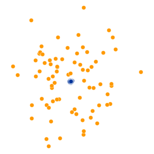
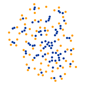
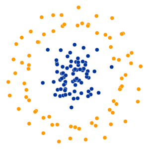
High perplexity \(\iff\) high entropy (eventually Gaussian ball will grow so big that all other points will be equally likely!). So, vary perplexity, see how plot changes
See here for an absolutely incredible interactive walkthrough of t-SNE!

What Happens As We Vary Perplexity?

Decision Trees

20 Questions

I am thinking of some entity. What is it?
What questions should we ask initially?
Why might questions on the left be more helpful than questions on the right?

General Questions	Specific Questions
Is it a physical object?	Is it a soda can?
Is it an animal?	Is it a cat?
Is it bigger than a house?	Is it a planet?

For linguistics fans: if a word \(x\) is one level “more general” than another word \(y\) (e.g., the word “camel” is one level more general than “bactrian camel”, a camel with two humps), we say that \(x\) is a hypernym of \(y\), and that \(y\) is a hyponym of \(x\). The WordNet project is a big tree of hypernym/hyponym relationships among all English words, where “entity” is the root node of the tree.

We Can Quantify How Good a Sequence of Questions Is!

Assume we’re playing with someone who only knows three objects \(S = \{\text{Tree}, \text{Bird}, \text{Car}\}\), and they randomize among these such that

\(\text{Choice}\)	Tree	Bird	Car
\(\Pr(\text{Choice})\)	0.25	0.25	0.50

Why might the “script” on the left be a better choice than script in the middle? Why are left and middle both better than right?

Example adapted from this essay by Simon DeDeo!

Let’s Use Math

An optimal script minimizes average number of questions required to reach answer

\[ \begin{align*} &\mathbb{E}[\text{\# Moves}] \\ =\,&1 \cdot \Pr(\text{Car}) + 2 \cdot \Pr(\text{Bird}) \\ &+ 2 \cdot \Pr(\text{Tree}) \\ =\,&1 \cdot 0.5 + 2\cdot 0.25 + 2\cdot 0.25 \\ =\,&1.5 \end{align*} \]

\[ \begin{align*} &\mathbb{E}[\text{\# Moves}] \\ =\,&1 \cdot \Pr(\text{Bird}) + 2 \cdot \Pr(\text{Car}) \\ &+ 2 \cdot \Pr(\text{Tree}) \\ =\,&1 \cdot 0.25 + 2\cdot 0.5 + 2\cdot 0.25 \\ =\,&1.75 \end{align*} \]

\[ \begin{align*} &\mathbb{E}[\text{\# Moves}] \\ =\,&1 \cdot \Pr(\text{Bird}) + 3 \cdot \Pr(\text{Car}) \\ &+ 3 \cdot \Pr(\text{Tree}) \\ =\,&1 \cdot 0.25 + 3\cdot 0.5 + 3\cdot 0.25 \\ =\,&2.5 \end{align*} \]

Let’s Use (Different) Math

Forgetting about the individual trees for a moment, let’s compute the entropy of the RV representing the opponent’s choice.
In general, if \(X\) represents the opponent’s choice and \(\mathcal{R}_X = \{1, 2, \ldots, N\}\), the entropy of \(X\) is:

\[ \begin{align*} H(X) &= -\sum_{i=1}^N \Pr(X = i)\log_2\Pr(X = i) \end{align*} \]

So in our case we have:

\[ \begin{align*} H(X) &= -\left[ \Pr(X = \text{Car}) \log_2\Pr(X = \text{Car}) \right. \\ &\phantom{= -[ } + \Pr(X = \text{Bird})\log_2\Pr(X = \text{Bird}) \\ &\phantom{= -[ } + \left. \Pr(X = \text{Tree})\log_2\Pr(X = \text{Tree})\right] \\ &= -\left[ (0.5)(-1) + (0.25)(-2) + (0.25)(-2) \right] = 1.5~🧐 \end{align*} \]

Entropy Seems Helpful Here…

Now let’s imagine our opponent randomizes between all three options:

\[ \begin{align*} \mathbb{E}[\text{\# Moves}] &= 1 \cdot (1/3) + 2 \cdot (1/3) + 2 \cdot (1/3) \\ &= \frac{5}{3} \approx 1.667 \end{align*} \]

\[ \begin{align*} H(X) &= -\left[ \Pr(X = \text{Car}) \log_2\Pr(X = \text{Car}) \right. \\ &\phantom{= -[ } + \Pr(X = \text{Bird})\log_2\Pr(X = \text{Bird}) \\ &\phantom{= -[ } + \left. \Pr(X = \text{Tree})\log_2\Pr(X = \text{Tree})\right] \\ &= -\left[ \frac{1}{3}\log_2\left(\frac{1}{3}\right) + \frac{1}{3}\log_2\left(\frac{1}{3}\right) + \frac{1}{3}\log_2\left(\frac{1}{3}\right) \right] \approx 1.585~🧐 \end{align*} \]

The Mathematical Relationship

The smallest possible number of levels \(L^*\) for a script based on RV \(X\) is exactly

\[ L^* = \lceil H(X) \rceil \]

Intuition: Although \(\mathbb{E}[\text{\# Moves}] = 1.5\), we cannot have a tree with 1.5 levels!
Entropy provides a lower bound on \(\mathbb{E}[\text{\# Moves}]\):

\[ \mathbb{E}[\text{\# Moves}] \geq H(X) \]

Decision Tree Structure

Leaf Nodes represent outcomes
Branch Nodes represent questions

How Are They Built?

Example: we find ourselves at some point on the globe, at some time during the year, and we’re trying to see whether this point+time are good for skiing

Code

library(tidyverse)
library(lubridate)
sample_size <- 100
day <- seq(ymd('2023-01-01'),ymd('2023-12-31'),by='weeks')
lat_bw <- 5
latitude <- seq(-90, 90, by=lat_bw)
ski_df <- expand_grid(day, latitude)
#ski_df |> head()
# Data-generating process
lat_cutoff <- 35
ski_df <- ski_df |> mutate(
  near_equator = abs(latitude) <= lat_cutoff,
  northern = latitude > lat_cutoff,
  southern = latitude < -lat_cutoff,
  first_3m = day < ymd('2023-04-01'),
  last_3m = day >= ymd('2023-10-01'),
  middle_6m = (day >= ymd('2023-04-01')) & (day < ymd('2023-10-01')),
  snowfall = 0
)
# Update the non-zero sections
mu_snow <- 10
sd_snow <- 2.5
# How many northern + first 3 months
num_north_first_3 <- nrow(ski_df[ski_df$northern & ski_df$first_3m,])
ski_df[ski_df$northern & ski_df$first_3m, 'snowfall'] = rnorm(num_north_first_3, mu_snow, sd_snow)
# Northerns + last 3 months
num_north_last_3 <- nrow(ski_df[ski_df$northern & ski_df$last_3m,])
ski_df[ski_df$northern & ski_df$last_3m, 'snowfall'] = rnorm(num_north_last_3, mu_snow, sd_snow)
# How many southern + middle 6 months
num_south_mid_6 <- nrow(ski_df[ski_df$southern & ski_df$middle_6m,])
ski_df[ski_df$southern & ski_df$middle_6m, 'snowfall'] = rnorm(num_south_mid_6, mu_snow, sd_snow)
# And collapse into binary var
ski_df['good_skiing'] = ski_df$snowfall > 0
# This converts day into an int
ski_df <- ski_df |> mutate(
  day_num = lubridate::yday(day)
)
#print(nrow(ski_df))
ski_sample <- ski_df |> slice_sample(n = sample_size)
ski_sample |> write_csv("assets/ski.csv")
ggplot(
  ski_sample,
  aes(
    x=day,
    y=latitude,
    #shape=good_skiing,
    color=good_skiing
  )) +
  geom_point(
    size = g_pointsize / 1.5,
    #stroke=1.5
  ) +
  dsan_theme() +
  labs(
    x = "Time of Year",
    y = "Latitude",
    shape = "Good Skiing?"
  ) +
  scale_shape_manual(name="Good Skiing?", values=c(1, 3)) +
  scale_color_manual(name="Good Skiing?", values=c(cbPalette[1], cbPalette[2]), labels=c("No (Sunny)","Yes (Snowy)")) +
  scale_x_continuous(
    breaks=c(ymd('2023-01-01'), ymd('2023-02-01'), ymd('2023-03-01'), ymd('2023-04-01'), ymd('2023-05-01'), ymd('2023-06-01'), ymd('2023-07-01'), ymd('2023-08-01'), ymd('2023-09-01'), ymd('2023-10-01'), ymd('2023-11-01'), ymd('2023-12-01')),
    labels=c("Jan", "Feb", "Mar", "Apr", "May", "Jun", "Jul", "Aug", "Sep", "Oct", "Nov", "Dec")
  ) +
  scale_y_continuous(breaks=c(-90, -60, -30, 0, 30, 60, 90))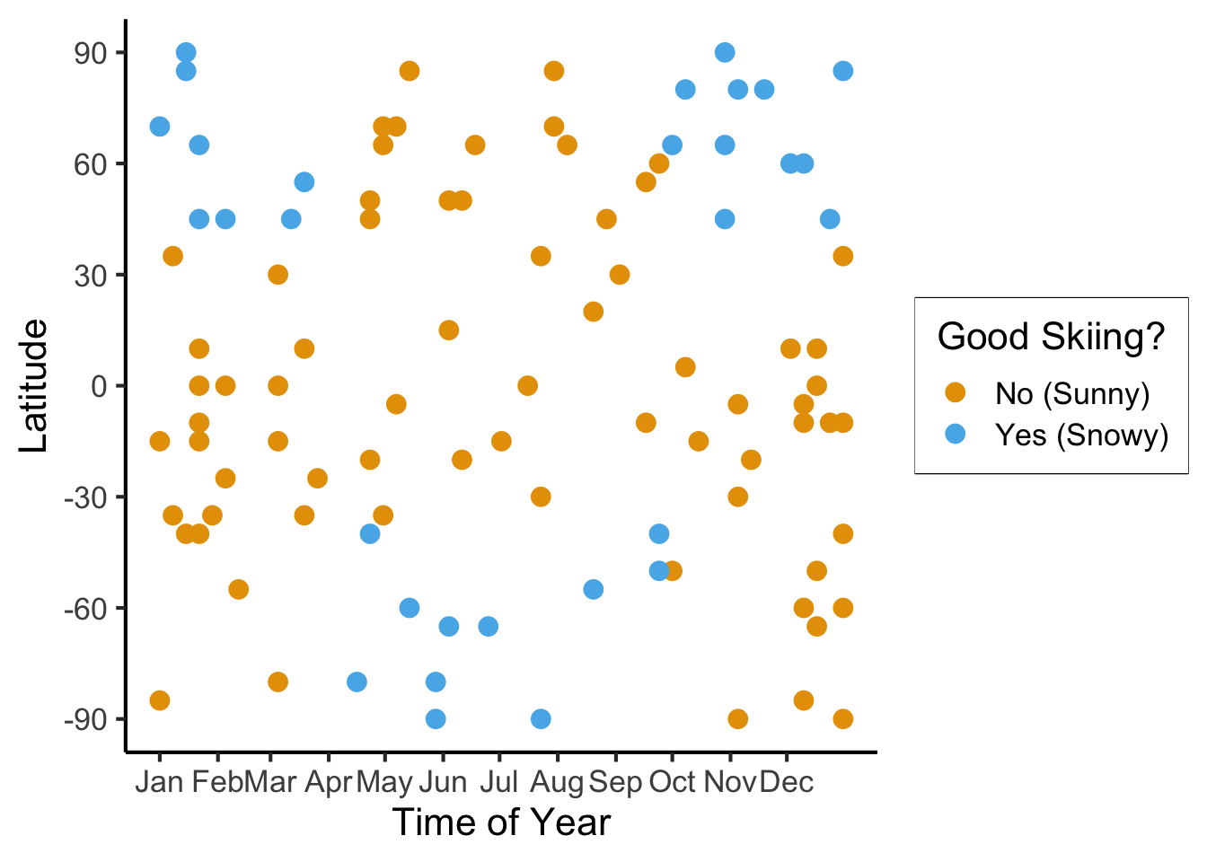

*(Example adapted from CS229: Machine Learning, Stanford University)*

Zero Splits

Starting out: no splits at all, just guess most frequent class: bad skiing

Code

ski_sample |> count(good_skiing)

good_skiing	n
FALSE	70
TRUE	30

This gives us \(\Pr(\text{Correct Guess}) = 0.66\)
Let \(R_i\) denote the region we’re considering at level \(i\), and \(\widehat{p}_c(R_i)\) be the proportion of points in region \(R_i\) that are of class \(c\)
The (nearly) unique measure is, you guessed it: entropy:

\[ \mathscr{L}(R_i) = -\sum_{c}\widehat{p}_c(R_i)\log_2(\widehat{p}_c(R_i)) \]

Here, since we’re not splitting the region up at all (yet), the entropy is just

\[ \mathscr{L}(R_i) = -[(0.66)\log_2(0.66) + (0.34)\log_2(0.34)] \approx 0.925 \]

Judging Split Options

Let’s think through two choices for the first split:

Code

ski_sample <- ski_sample |> mutate(
  lat_lt_475 = latitude <= 47.5
)
ski_sample |> group_by(lat_lt_475) |> count(good_skiing)
ski_sample <- ski_sample |> mutate(
  month_lt_oct = day < ymd('2023-10-01')
)
ski_sample |> group_by(month_lt_oct) |> count(good_skiing)

\(\text{latitude} \leq -47.5\):

lat_lt_475	good_skiing	n
FALSE	FALSE	13
FALSE	TRUE	14
TRUE	FALSE	57
TRUE	TRUE	16

This gives us the rule

\[ \widehat{C}(x) = \begin{cases} 0 &\text{if }\text{latitude} \leq 47.5, \\ 0 &\text{otherwise} \end{cases} \]

\(\text{month} < \text{October}\)

month_lt_oct	good_skiing	n
FALSE	FALSE	22
FALSE	TRUE	11
TRUE	FALSE	48
TRUE	TRUE	19

This gives us the rule

\[ \widehat{C}(x) = \begin{cases} 0 &\text{if }\text{month} < \text{October}, \\ 0 &\text{otherwise} \end{cases} \]

So, if we judge purely on acuracy scores… it seems like we’re not getting anywhere here (but, we know we are getting somewhere!)

Scikit-Learn: Growing the Tree

Code

import json
import pandas as pd
import numpy as np
import sklearn
from sklearn.tree import DecisionTreeClassifier
sklearn.set_config(display='text')
ski_df = pd.read_csv("assets/ski.csv")
ski_df['good_skiing'] = ski_df['good_skiing'].astype(int)
X = ski_df[['day_num', 'latitude']]
y = ski_df['good_skiing']
dtc = DecisionTreeClassifier(
  max_depth = 1,
  criterion = "entropy"
)
dtc.fit(X, y);
y_pred = pd.Series(dtc.predict(X), name="y_pred")
result_df = pd.concat([X,y,y_pred], axis=1)
result_df['correct'] = result_df['good_skiing'] == result_df['y_pred']
result_df.to_csv("assets/ski_predictions.csv")
sklearn.tree.plot_tree(dtc, feature_names = X.columns)
n_nodes = dtc.tree_.node_count
children_left = dtc.tree_.children_left
children_right = dtc.tree_.children_right
feature = dtc.tree_.feature
feat_index = feature[0]
feat_name = X.columns[feat_index]
thresholds = dtc.tree_.threshold
feat_threshold = thresholds[0]
#print(f"Feature: {feat_name}\nThreshold: <= {feat_threshold}")
values = dtc.tree_.value
#print(values)
dt_data = {
  'feat_index': feat_index,
  'feat_name': feat_name,
  'feat_threshold': feat_threshold
}
dt_df = pd.DataFrame([dt_data])
dt_df.to_feather('assets/ski_dt.feather')
library(tidyverse)
library(arrow)
# Load the dataset
ski_result_df <- read_csv("assets/ski_predictions.csv")
# Load the DT info
dt_df <- read_feather("assets/ski_dt.feather")
# Here we only have one value, so just read that
# value directly
lat_thresh <- dt_df$feat_threshold
ggplot(ski_result_df, aes(x=day_num, y=latitude, color=factor(good_skiing), shape=correct)) +
  geom_point(
    size = g_pointsize / 1.5,
    stroke = 1.5
  ) +
  geom_hline(
    yintercept = lat_thresh,
    linetype = "dashed"
  ) +
  dsan_theme("half") +
  labs(
    x = "Time of Year",
    y = "Latitude",
    color = "True Class",
    #shape = "Correct?"
  ) +
  scale_shape_manual("DT Prediction", values=c(1,3), labels=c("Incorrect","Correct")) +
  scale_color_manual("True Class", values=c(cbPalette[1], cbPalette[2]), labels=c("Bad (Sunny)","Good (Snowy)"))
ski_result_df |> count(correct)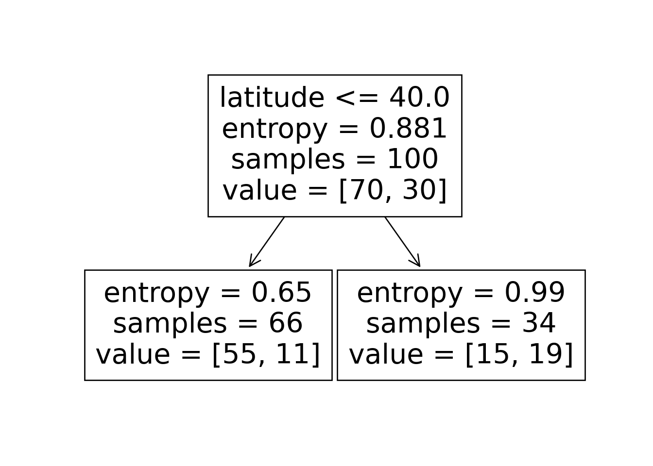

The Estimated Tree:

Performance:


Attaching package: 'arrow'

The following object is masked from 'package:lubridate':

    duration

The following object is masked from 'package:utils':

    timestamp

New names:
• `` -> `...1`

Rows: 100 Columns: 6
── Column specification ────────────────────────────────────────────────────────
Delimiter: ","
dbl (5): ...1, day_num, latitude, good_skiing, y_pred
lgl (1): correct

ℹ Use `spec()` to retrieve the full column specification for this data.
ℹ Specify the column types or set `show_col_types = FALSE` to quiet this message.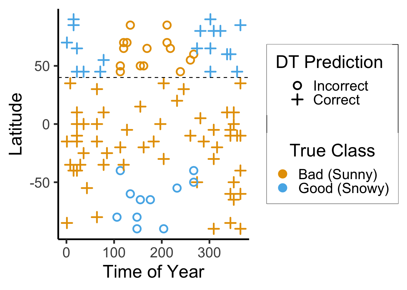

correct	n
FALSE	26
TRUE	74

\[ \begin{align*} \mathscr{L}(R_1) &= -\left[ \frac{13}{25}\log_2\left(\frac{13}{25}\right) + \frac{12}{25}\log_2\left(\frac{12}{25}\right) \right] \approx 0.999 \\ \mathscr{L}(R_2) &= -\left[ \frac{61}{75}\log_2\left(\frac{61}{75}\right) + \frac{14}{75}\log_2\left(\frac{14}{75}\right) \right] \approx 0.694 \\ %\mathscr{L}(R \rightarrow (R_1, R_2)) &= \Pr(x_i \in R_1)\mathscr{L}(R_1) + \Pr(x_i \in R_2)\mathscr{L}(R_2) \\ \mathscr{L}(R_1, R_2) &= \frac{1}{4}(0.999) + \frac{3}{4}(0.694) \approx 0.77 < 0.827~😻 \end{align*} \]

Chopping the Feature Space Always Reduces Entropy (!)

Visual proof:

Code

library(tidyverse)
my_ent <- function(x) -(x * log2(x) + (1-x)*log2(1-x))
loss_df <- tribble(
  ~x, ~label,
  0.5, "L(R1)",
  0.9, "L(R2)",
  0.7, "L(R)"
)
loss_df <- loss_df |> mutate(
  y = my_ent(x)
)
ggplot(data=tibble(x=c(0,1))) +
  stat_function(fun=my_ent, linewidth = g_linewidth) +
  geom_text(data=loss_df, aes(x=x, y=y, label=label)) +
  xlim(c(0,1)) +
  dsan_theme("half")

Warning: Removed 2 rows containing missing values or values outside the scale range
(`geom_function()`).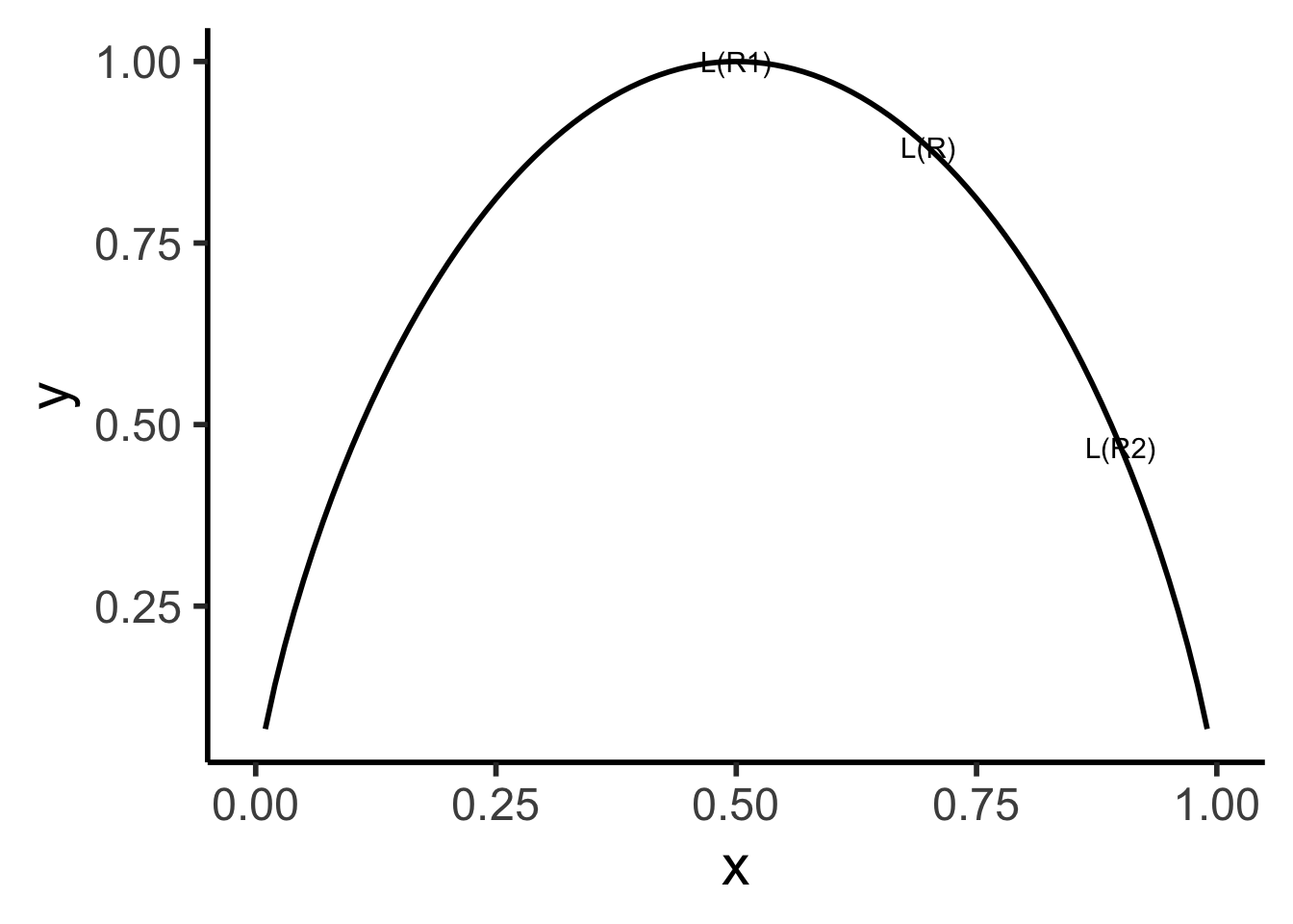

Continuous Values

What if we replace binary labels with continuous values: in this case, cm of snow?

Code

#format_snow <- function(x) sprintf('%.2f', x)
format_snow <- function(x) round(x, 2)
ski_sample['snowfall_str'] <- sapply(ski_sample$snowfall, format_snow)
#ski_df |> head()
#print(nrow(ski_df))
ggplot(ski_sample, aes(x=day, y=latitude, label=snowfall_str)) +
  geom_text(size = 6) +
  dsan_theme() +
  labs(
    x = "Time of Year",
    y = "Latitude",
    shape = "Good Skiing?"
  ) +
  scale_shape_manual(values=c(1, 3)) +
  scale_x_continuous(
    breaks=c(ymd('2023-01-01'), ymd('2023-02-01'), ymd('2023-03-01'), ymd('2023-04-01'), ymd('2023-05-01'), ymd('2023-06-01'), ymd('2023-07-01'), ymd('2023-08-01'), ymd('2023-09-01'), ymd('2023-10-01'), ymd('2023-11-01'), ymd('2023-12-01')),
    labels=c("Jan", "Feb", "Mar", "Apr", "May", "Jun", "Jul", "Aug", "Sep", "Oct", "Nov", "Dec")
  ) +
  scale_y_continuous(breaks=c(-90, -60, -30, 0, 30, 60, 90))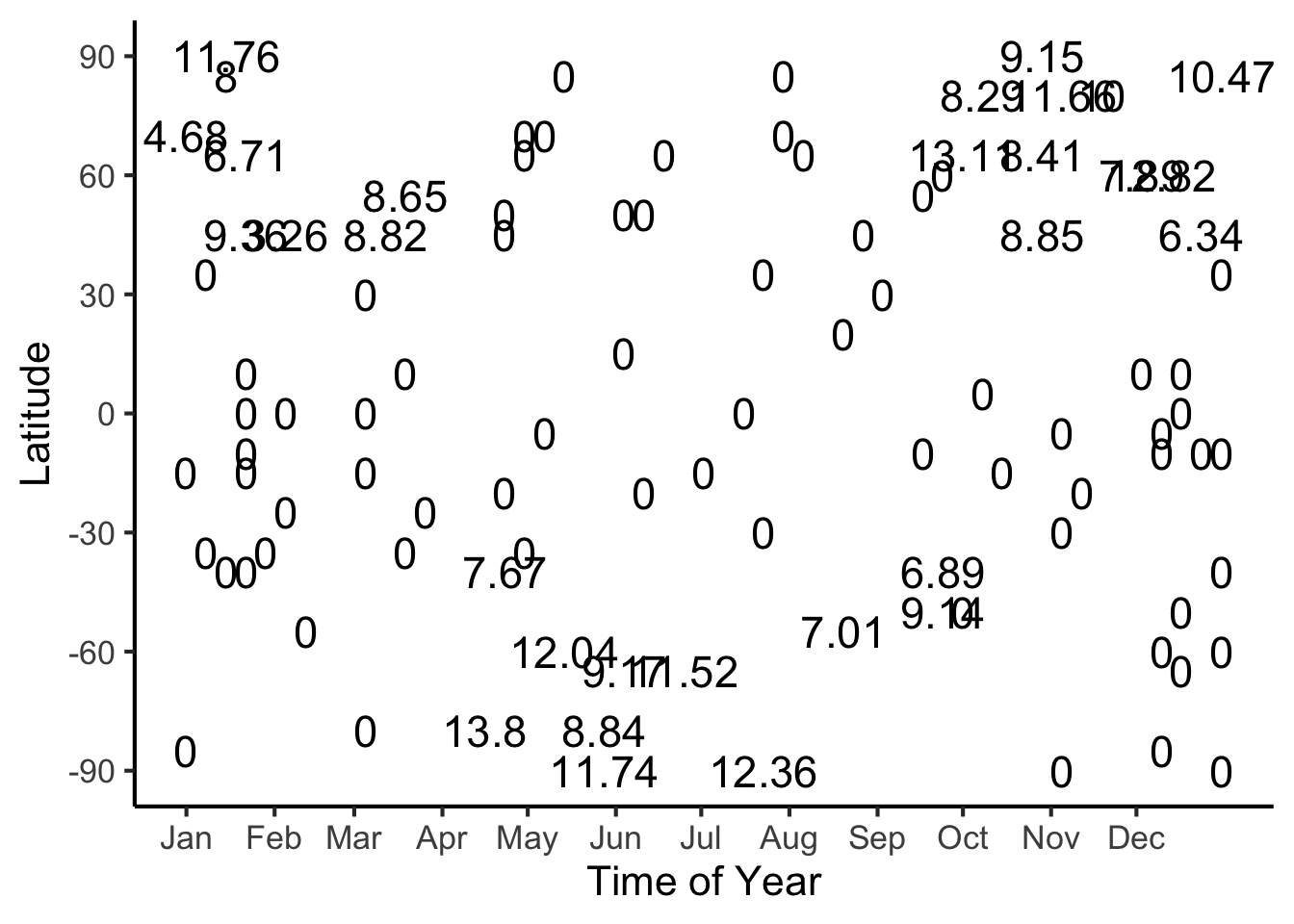

Looking Towards Regression

How could we make a decision tree to predict \(y\) from \(x\) for this data?

Code

library(tidyverse)
library(latex2exp)
expr_pi2 <- TeX("$\\frac{\\pi}{2}$")
expr_pi <- TeX("$\\pi$")
expr_3pi2 <- TeX("$\\frac{3\\pi}{2}$")
expr_2pi <- TeX("$2\\pi$")
x_range <- 2 * pi
x_coords <- seq(0, x_range, by = x_range / 100)
num_x_coords <- length(x_coords)
data_df <- tibble(x = x_coords)
data_df <- data_df |> mutate(
  y_raw = sin(x),
  y_noise = rnorm(num_x_coords, 0, 0.15)
)
data_df <- data_df |> mutate(
  y = y_raw + y_noise
)
#y_coords <- y_raw_coords + y_noise
#y_coords <- y_raw_coords
#data_df <- tibble(x = x, y = y)
reg_tree_plot <- ggplot(data_df, aes(x=x, y=y)) +
  geom_point(size = g_pointsize / 2) +
  dsan_theme("half") +
  labs(
    x = "Feature",
    y = "Label"
  ) +
  geom_vline(
    xintercept = pi,
    linewidth = g_linewidth,
    linetype = "dashed"
  ) +
  scale_x_continuous(
    breaks=c(0,pi/2,pi,(3/2)*pi,2*pi),
    labels=c("0",expr_pi2,expr_pi,expr_3pi2,expr_2pi)
  )
reg_tree_plot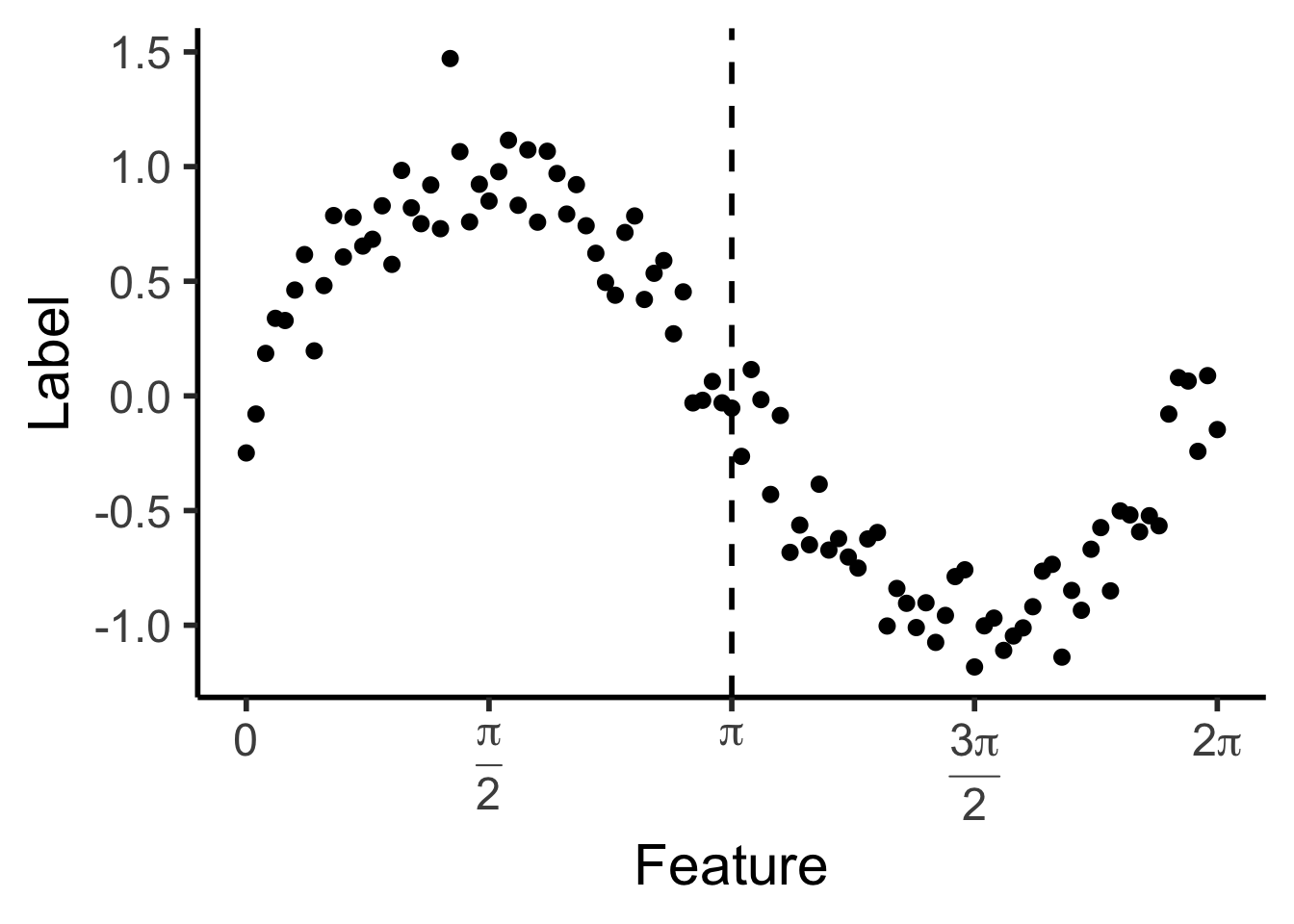

A Zero-Level Tree

Trivial example: \(\widehat{y}(x) = 0\). How well does this do?

Code

library(ggtext)
# x_lt_pi = data_df |> filter(x < pi)
# mean(x_lt_pi$y)
data_df <- data_df |> mutate(
  pred_sq_err0 = (y - 0)^2
)
mse0 <- mean(data_df$pred_sq_err0)
mse0_str <- sprintf("%.3f", mse0)
reg_tree_plot +
  geom_hline(
    yintercept = 0,
    color=cbPalette[1],
    linewidth = g_linewidth
  ) +
  geom_segment(
    aes(x=x, xend=x, y=0, yend=y)
  ) +
  geom_text(
    aes(x=(3/2)*pi, y=0.5, label=paste0("MSE = ",mse0_str)),
    size = 10,
    #box.padding = unit(c(2,2,2,2), "pt")
  )

Warning in geom_text(aes(x = (3/2) * pi, y = 0.5, label = paste0("MSE = ", : All aesthetics have length 1, but the data has 101 rows.
ℹ Please consider using `annotate()` or provide this layer with data containing
  a single row.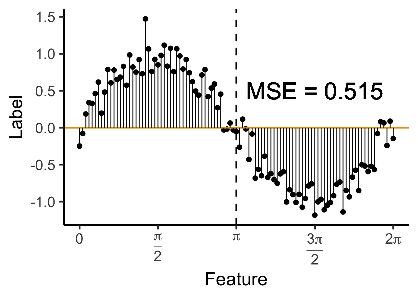

A One-Level Binary Tree

Let’s introduce a single branch node:

\[ \widehat{y}(x) = \begin{cases} \phantom{-}\frac{2}{\pi} &\text{if }x < \pi, \\ -\frac{2}{\pi} &\text{otherwise.} \end{cases} \]

Code

get_y_pred <- function(x) ifelse(x < pi, 2/pi, -2/pi)
data_df <- data_df |> mutate(
  pred_sq_err1 = (y - get_y_pred(x))^2
)
mse1 <- mean(data_df$pred_sq_err1)
mse1_str <- sprintf("%.3f", mse1)
decision_df <- tribble(
  ~x, ~xend, ~y, ~yend,
  0, pi, 2/pi, 2/pi,
  pi, 2*pi, -2/pi, -2/pi
)
reg_tree_plot +
  geom_segment(
    data=decision_df,
    aes(x=x, xend=xend, y=y, yend=yend),
    color=cbPalette[1],
    linewidth = g_linewidth
  ) +
  geom_segment(
    aes(x=x, xend=x, y=get_y_pred(x), yend=y)
  ) +
  geom_text(
    aes(x=(3/2)*pi, y=0.5, label=paste0("MSE = ",mse1_str)),
    size = 9,
    #box.padding = unit(c(2,2,2,2), "pt")
  )

Warning in geom_text(aes(x = (3/2) * pi, y = 0.5, label = paste0("MSE = ", : All aesthetics have length 1, but the data has 101 rows.
ℹ Please consider using `annotate()` or provide this layer with data containing
  a single row.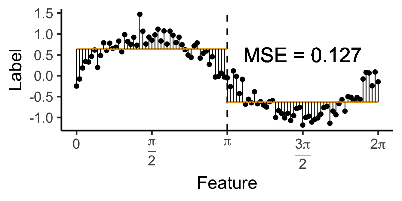

A One-Level Ternary Tree

Now let’s allow three answers:

\[ \widehat{y}(x) = \begin{cases} \phantom{-}\frac{9}{4\pi} &\text{if }x < \frac{2\pi}{3}, \\ \phantom{-}0 &\text{if }\frac{2\pi}{3} \leq x \leq \frac{4\pi}{3} \\ -\frac{9}{4\pi} &\text{otherwise.} \end{cases} \]

Code

cut1 <- (2/3) * pi
cut2 <- (4/3) * pi
pos_mean <- 9 / (4*pi)
get_y_pred <- function(x) ifelse(x < cut1, pos_mean, ifelse(x < cut2, 0, -pos_mean))
data_df <- data_df |> mutate(
  pred_sq_err1b = (y - get_y_pred(x))^2
)
mse1b <- mean(data_df$pred_sq_err1b)
mse1b_str <- sprintf("%.3f", mse1b)
decision_df <- tribble(
  ~x, ~xend, ~y, ~yend,
  0, (2/3)*pi, pos_mean, pos_mean,
  (2/3)*pi, (4/3)*pi, 0, 0,
  (4/3)*pi, 2*pi, -pos_mean, -pos_mean
)
reg_tree_plot +
  geom_segment(
    data=decision_df,
    aes(x=x, xend=xend, y=y, yend=yend),
    color=cbPalette[1],
    linewidth = g_linewidth
  ) +
  geom_segment(
    aes(x=x, xend=x, y=get_y_pred(x), yend=y)
  ) +
  geom_text(
    aes(x=(3/2)*pi, y=0.5, label=paste0("MSE = ",mse1b_str)),
    size = 9,
    #box.padding = unit(c(2,2,2,2), "pt")
  )

Warning in geom_text(aes(x = (3/2) * pi, y = 0.5, label = paste0("MSE = ", : All aesthetics have length 1, but the data has 101 rows.
ℹ Please consider using `annotate()` or provide this layer with data containing
  a single row.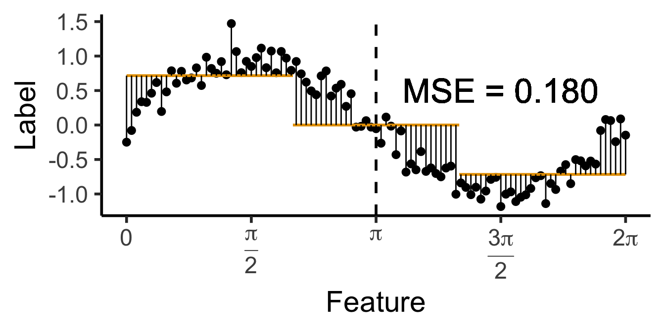

Another One-Level Ternary Tree

Now let’s allow an uneven split:

\[ \widehat{y}(x) = \begin{cases} \phantom{-}0.695 &\text{if }x < (1-c)\pi, \\ \phantom{-}0 &\text{if }(1-c)\pi \leq x \leq (1+c)\pi \\ -0.695 &\text{otherwise,} \end{cases} \]

with \(c \approx 0.113\), gives us:

Code

c <- 0.113
cut1 <- (1 - c) * pi
cut2 <- (1 + c) * pi
pos_mean <- 0.695
get_y_pred <- function(x) ifelse(x < cut1, pos_mean, ifelse(x < cut2, 0, -pos_mean))
data_df <- data_df |> mutate(
  pred_sq_err1b = (y - get_y_pred(x))^2
)
mse1b <- mean(data_df$pred_sq_err1b)
mse1b_str <- sprintf("%.3f", mse1b)
decision_df <- tribble(
  ~x, ~xend, ~y, ~yend,
  0, cut1, pos_mean, pos_mean,
  cut1, cut2, 0, 0,
  cut2, 2*pi, -pos_mean, -pos_mean
)
reg_tree_plot +
  geom_segment(
    data=decision_df,
    aes(x=x, xend=xend, y=y, yend=yend),
    color=cbPalette[1],
    linewidth = g_linewidth
  ) +
  geom_segment(
    aes(x=x, xend=x, y=get_y_pred(x), yend=y)
  ) +
  geom_text(
    aes(x=(3/2)*pi, y=0.5, label=paste0("MSE = ",mse1b_str)),
    size = 9,
    #box.padding = unit(c(2,2,2,2), "pt")
  )

Warning in geom_text(aes(x = (3/2) * pi, y = 0.5, label = paste0("MSE = ", : All aesthetics have length 1, but the data has 101 rows.
ℹ Please consider using `annotate()` or provide this layer with data containing
  a single row.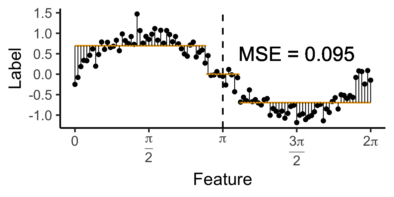

On to the Code!

Scikit-learn has both DecisionTreeClassifier and DecisionTreeRegressor classes!

Appendix: Covariance Matrix Magic

For those interested (skipping over lots of matrix math): say you have a 2D covariance matrix \(\mathbf{\Sigma}\) with eigensystem \((\lambda_1, \mathbf{x}_1), (\lambda_2, \mathbf{x}_2)\)
You can obtain a new covariance matrix \(\mathbf{\Sigma}'\) which has the same eigenvalues as \(\mathbf{\Sigma}\) but has eigenvectors \(\mathbf{x}'_1\) and \(\mathbf{x}'_2\), so long as these two eigenvectors are orthogonal.
Example: you want to retain the eigenvalues \(\lambda_1 = 3\) and \(\lambda_2 = 1\) from the quiz-review slides, but want the data’s first principal component to be \(\mathbf{x}'_1 = (2,1)^\top\) and its second principal component to be \(\mathbf{x}'_2 = (-1,2)^\top\).
By constructing the Eigenmatrix \(\mathbf{V} = \left[\begin{smallmatrix} \mathbf{x}'_1 & \mathbf{x}'_2\end{smallmatrix}\right]\) (the matrix whose columns are \(\mathbf{x}'_1\) and \(\mathbf{x}'_2\)), we can obtain \(\mathbf{\Sigma}'\) by computing:

\[ \mathbf{\Sigma}' = \mathbf{V}\mathbf{\Sigma}\mathbf{V}^{-1}. \]

(Exercise: recreate the plot from the earlier PCA slides, but with these desired first and second principal components! See here for a deeper dive into why this works!)

References

Van der Maaten, Laurens, and Geoffrey Hinton. 2008. “Visualizing Data Using t-SNE.” Journal of Machine Learning Research 9 (11).