- Decision Trees
Week 13: Course Wrapup
DSAN 5000: Data Science and Analytics
Thursday, December 5, 2024
Student Presentations
Code
cb_palette = ["#E69F00", "#56B4E9", "#009E73", "#F0E442", "#0072B2", "#D55E00", "#CC79A7"]

from IPython.display import Markdown
def disp(df, floatfmt='g', include_index=True):
  return Markdown(
    df.to_markdown(
      floatfmt=floatfmt,
      index=include_index
    )
  )

def summary_to_df(summary_obj, corner_col = ''):
    reg_df = pd.DataFrame(summary_obj.tables[1].data)
    reg_df.columns = reg_df.iloc[0]
    reg_df = reg_df.iloc[1:].copy()
    # Save index col
    index_col = reg_df['']
    # Drop for now, so it's all numeric
    reg_df.drop(columns=[''], inplace=True)
    reg_df = reg_df.apply(pd.to_numeric)
    my_round = lambda x: round(x, 2)
    reg_df = reg_df.apply(my_round)
    numeric_cols = reg_df.columns
    # Add index col back in
    reg_df.insert(loc=0, column=corner_col, value=index_col)
    # Sigh. Have to escape | characters?
    reg_df.columns = [c.replace("|","\|") for c in reg_df.columns]
    return reg_df
\[ \DeclareMathOperator*{\argmax}{argmax} \DeclareMathOperator*{\argmin}{argmin} \newcommand{\bigexpect}[1]{\mathbb{E}\mkern-4mu \left[ #1 \right]} \newcommand{\definedas}{\overset{\text{defn}}{=}} \newcommand{\definedalign}{\overset{\phantom{\text{defn}}}{=}} \newcommand{\eqeventual}{\overset{\text{eventually}}{=}} \newcommand{\expect}[1]{\mathbb{E}[#1]} \newcommand{\expectsq}[1]{\mathbb{E}^2[#1]} \newcommand{\fw}[1]{\texttt{#1}} \newcommand{\given}{\mid} \newcommand{\green}[1]{\color{green}{#1}} \newcommand{\heads}{\outcome{heads}} \newcommand{\iqr}{\text{IQR}} \newcommand{\kl}{\text{KL}} \newcommand{\lik}{\mathcal{L}} \newcommand{\mle}{\textsf{ML}} \newcommand{\orange}[1]{\color{orange}{#1}} \newcommand{\outcome}[1]{\textsf{#1}} \newcommand{\param}[1]{{\color{purple} #1}} \newcommand{\paramDist}{\param{\boldsymbol\theta_\mathcal{D}}} \newcommand{\pgsamplespace}{\{\green{1},\green{2},\green{3},\purp{4},\purp{5},\purp{6}\}} \newcommand{\prob}[1]{P\left( #1 \right)} \newcommand{\purp}[1]{\color{purple}{#1}} \newcommand{\red}[1]{\color{red}#1} \newcommand{\spacecap}{\; \cap \;} \newcommand{\spacewedge}{\; \wedge \;} \newcommand{\tails}{\outcome{tails}} \newcommand{\Var}[1]{\text{Var}[#1]} \newcommand{\bigVar}[1]{\text{Var}\mkern-4mu \left[ #1 \right]} \]
Course Recap

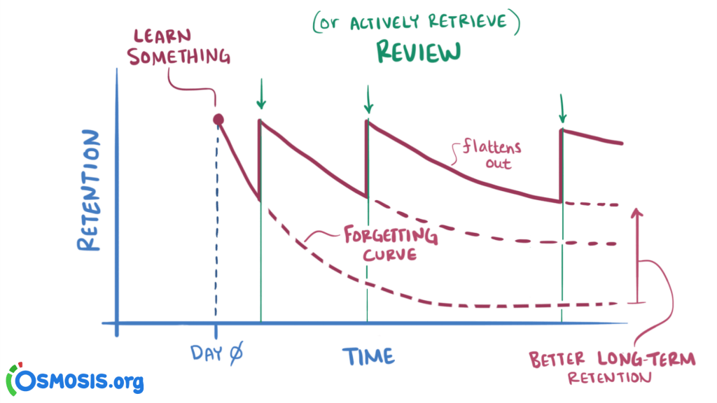
(Why Do A Course Recap?)
Data = Ground Truth + Noise
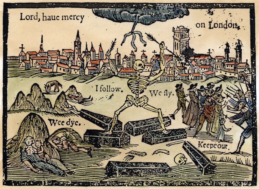
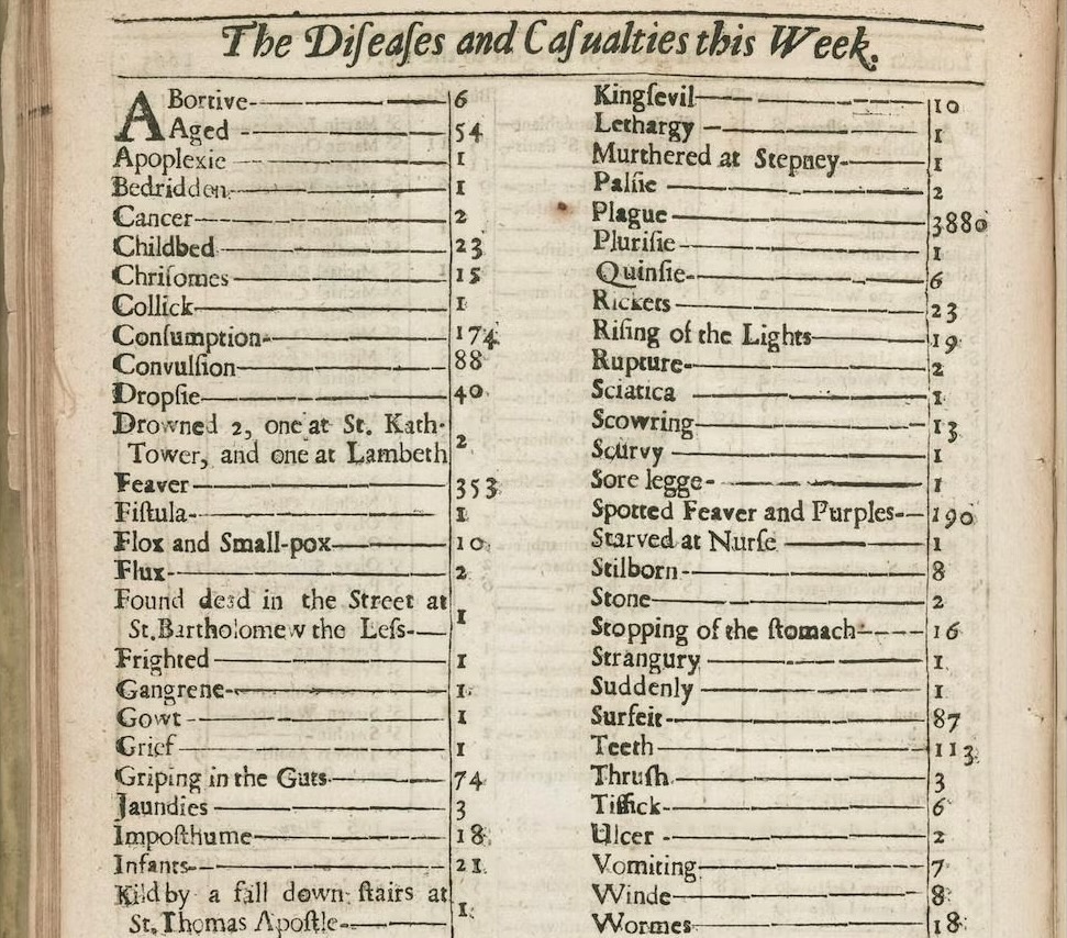
- Depressing but true origin of statistics (as opposed to probability): the Plague 😷
Your Toolbox
- GitHub
- File Formats
- Web Scraping
- Data-Generating Processes (DGPs)
- Distance Metrics
- Entropy
- Gaussian / Normal Distributions
- Clustering
- Dimensionality Reduction
GitHub (W03)
Data Structures: Simple \(\rightarrow\) Complex (W04)
| id | name | |
|---|---|---|
| 0 | K. Desbrow | kd9@dailymail.com |
| 1 | D. Minall | dminall1@wired.com |
| 2 | C. Knight | ck2@microsoft.com |
| 3 | M. McCaffrey | mccaf4@nhs.uk |
| year | month | points |
|---|---|---|
| 2023 | Jan | 65 |
| 2023 | Feb | |
| 2023 | Mar | 42 |
| 2023 | Apr | 11 |
| id | date | rating | num_rides |
|---|---|---|---|
| 0 | 2023-01 | 0.75 | 45 |
| 0 | 2023-02 | 0.89 | 63 |
| 0 | 2023-03 | 0.97 | 7 |
| 1 | 2023-06 | 0.07 | 10 |
| id | Source | Target | Weight |
|---|---|---|---|
| 1 | IGF2 | IGF1R | 1 |
| 2 | IGF1R | TP53 | 2 |
| 3 | TP53 | EGFR | 0.5 |
Web Scraping (W04)
| How is data loaded? | Solution | Example | ||
|---|---|---|---|---|
| 😊 | Easy | Data in HTML source | “View Source” | |
| 😐 | Medium | Data loaded dynamically via API | “View Source”, find API call, scrape programmatically | |
| 😳 | Hard | Data loaded dynamically [internally] via web framework | Use Selenium |
EDA: Why We Can’t Just Skip It (W06)
- Iterative process: Ask questions of the data, find answers, generate more questions
- You’re probably already used to Mean and Variance: Fancier EDA/robustness methods build upon these two!
- Why do we need to visualize? Can’t we just use mean, \(R^2\)?
- …Enter Anscombe’s Quartet
Code
import pandas as pd
import numpy as np
import matplotlib.pyplot as plt
import seaborn as sns
sns.set_theme(style="ticks")
# https://towardsdatascience.com/how-to-use-your-own-color-palettes-with-seaborn-a45bf5175146
sns.set_palette(sns.color_palette(cb_palette))

# Load the example dataset for Anscombe's quartet
anscombe_df = sns.load_dataset("anscombe")
#print(anscombe_df)

# Show the results of a linear regression within each dataset
anscombe_plot = sns.lmplot(
    data=anscombe_df, x="x", y="y", col="dataset", hue="dataset",
    col_wrap=4, palette="muted", ci=None,
    scatter_kws={"s": 50, "alpha": 1},
    height=3
);
anscombe_plot;
The Scariest Dataset of All Time

Code
| dataset | x_mean | y_mean |
|---|---|---|
| I | 9.00 | 7.50 |
| II | 9.00 | 7.50 |
| III | 9.00 | 7.50 |
| IV | 9.00 | 7.50 |
Code
| x | y | ||
|---|---|---|---|
| dataset | |||
| I | x | 1.00 | 0.82 |
| y | 0.82 | 1.00 | |
| II | x | 1.00 | 0.82 |
| y | 0.82 | 1.00 | |
| III | x | 1.00 | 0.82 |
| y | 0.82 | 1.00 | |
| IV | x | 1.00 | 0.82 |
| y | 0.82 | 1.00 |
It Doesn’t End There…

Code
import statsmodels.formula.api as smf
summary_dfs = []
for cur_ds in ['I','II','III','IV']:
  ds1_df = anscombe_df.loc[anscombe_df['dataset'] == "I"].copy()
  # Fit regression model (using the natural log of one of the regressors)
  results = smf.ols('y ~ x', data=ds1_df).fit()
  # Get R^2
  rsq = round(results.rsquared, 2)
  # Inspect the results
  summary = results.summary()
  summary.extra_txt = None
  summary_df = summary_to_df(summary, corner_col = f'Dataset {cur_ds}<br>R^2 = {rsq}')
  summary_dfs.append(summary_df)
disp(summary_dfs[0], include_index=False)
disp(summary_dfs[1], include_index=False)
disp(summary_dfs[2], include_index=False)
disp(summary_dfs[3], include_index=False)| Dataset I R^2 = 0.67 |
coef | std err | t | P>|t| | [0.025 | 0.975] |
|---|---|---|---|---|---|---|
| Intercept | 3 | 1.12 | 2.67 | 0.03 | 0.46 | 5.54 |
| x | 0.5 | 0.12 | 4.24 | 0 | 0.23 | 0.77 |
| Dataset II R^2 = 0.67 |
coef | std err | t | P>|t| | [0.025 | 0.975] |
|---|---|---|---|---|---|---|
| Intercept | 3 | 1.12 | 2.67 | 0.03 | 0.46 | 5.54 |
| x | 0.5 | 0.12 | 4.24 | 0 | 0.23 | 0.77 |
| Dataset III R^2 = 0.67 |
coef | std err | t | P>|t| | [0.025 | 0.975] |
|---|---|---|---|---|---|---|
| Intercept | 3 | 1.12 | 2.67 | 0.03 | 0.46 | 5.54 |
| x | 0.5 | 0.12 | 4.24 | 0 | 0.23 | 0.77 |
| Dataset IV R^2 = 0.67 |
coef | std err | t | P>|t| | [0.025 | 0.975] |
|---|---|---|---|---|---|---|
| Intercept | 3 | 1.12 | 2.67 | 0.03 | 0.46 | 5.54 |
| x | 0.5 | 0.12 | 4.24 | 0 | 0.23 | 0.77 |
Naïve Bayes (W07)
Guessing House Prices:
- If I tell you there’s a house, what is your guess for number of bathrooms it has?
- If I tell you the house is 50,000 sqft, does your guess go up?
Guessing Word Frequencies:
- If I tell you there’s a book, how often do you think the word “University” appears?
- Now if I tell you that the word “Stanford” appears 2,000 times, does your guess go up?

In Math
- Assume some email \(E\) with \(N = 5\) words, \(E = (w_1, w_2, w_3, w_4, w_5)\). Say \(E = (\texttt{you},\texttt{win},\texttt{a},\texttt{million},\texttt{dollars})\).
- We’re trying to classify \(S = \begin{cases}1 &\text{if spam} \\ 0 &\text{otherwise}\end{cases}\) given \(E\)
- Normal person (marine biologist?)1:
\[ \begin{align*} &\Pr(S = 1 \mid w_5 = \texttt{dollars}, w_4 = \texttt{million}) \\ &> \Pr(S = 1 \mid w_5 = \texttt{dollars}, w_4 = \texttt{octopus}) \end{align*} \]
- Naïve Bayes classifier:
\[ \Pr(S = 1 \mid w_5) \perp \Pr(S = 1 \mid w_4) \]
Clutering (W09)
- Let \(\boldsymbol\mu_1 = (0.2, 0.8)^\top\), \(\boldsymbol\mu_2 = (0.8, 0.2)^\top\), \(\Sigma = \text{diag}(1/64)\), and \(\mathbf{X} = (X_1, X_2)\).
- \(X_1 \sim \boldsymbol{\mathcal{N}}_2(\boldsymbol\mu_1, \Sigma)\), \(X_2 \sim \boldsymbol{\mathcal{N}}_2(\boldsymbol\mu_2, \Sigma)\)
Code
library(tidyverse)
library(ggforce)
library(MASS)
library(patchwork)
N <- 50
Mu1 <- c(0.2, 0.8)
Mu2 <- c(0.8, 0.2)
sigma <- 1/24
# Data for concentric circles
circle_df <- tribble(
  ~x0, ~y0, ~r, ~Cluster, ~whichR,
  Mu1[1], Mu1[2], sqrt(sigma), "C1", 1,
  Mu2[1], Mu2[2], sqrt(sigma), "C2", 1,
  Mu1[1], Mu1[2], 2 * sqrt(sigma), "C1", 2,
  Mu2[1], Mu2[2], 2 * sqrt(sigma), "C2", 2,
  Mu1[1], Mu1[2], 3 * sqrt(sigma), "C1", 3,
  Mu2[1], Mu2[2], 3 * sqrt(sigma), "C2", 3
)
#print(circle_df)
Sigma <- matrix(c(sigma,0,0,sigma), nrow=2)
#print(Sigma)
x1_df <- as_tibble(mvrnorm(N, Mu1, Sigma))
x1_df <- x1_df |> mutate(
  Cluster='C1'
)
x2_df <- as_tibble(mvrnorm(N, Mu2, Sigma))
x2_df <- x2_df |> mutate(
  Cluster='C2'
)
cluster_df <- bind_rows(x1_df, x2_df)
cluster_df <- cluster_df |> rename(
  x=V1, y=V2
)
known_plot <- ggplot(cluster_df) +
  geom_point(
    data = circle_df,
    aes(x=x0, y=y0)
  ) +
  geom_circle(
    data = circle_df,
    aes(x0=x0, y0=y0, r=r, fill=Cluster),
    linewidth = g_linewidth,
    alpha = 0.25
  ) +
  geom_point(
    data=cluster_df,
    aes(x=x, y=y, fill=Cluster),
    size = g_pointsize / 2,
    shape = 21
  ) +
  dsan_theme("full") +
  coord_fixed() +
  labs(
    x = "x",
    y = "y",
    title = "Data with Known Clusters"
  ) +
  scale_fill_manual(values=c(cbPalette[2], cbPalette[1], cbPalette[3], cbPalette[4])) +
  scale_color_manual(values=c(cbPalette[1], cbPalette[2], cbPalette[3], cbPalette[4]))
unknown_plot <- ggplot(cluster_df) +
  geom_point(
    data=cluster_df,
    aes(x=x, y=y),
    size = g_pointsize / 2,
    #shape = 21
  ) +
  dsan_theme("full") +
  coord_fixed() +
  labs(
    x = "x",
    y = "y",
    title = "Same Data with Unknown Clusters"
  )
cluster_df |> write_csv("assets/cluster_data.csv")
known_plot + unknown_plot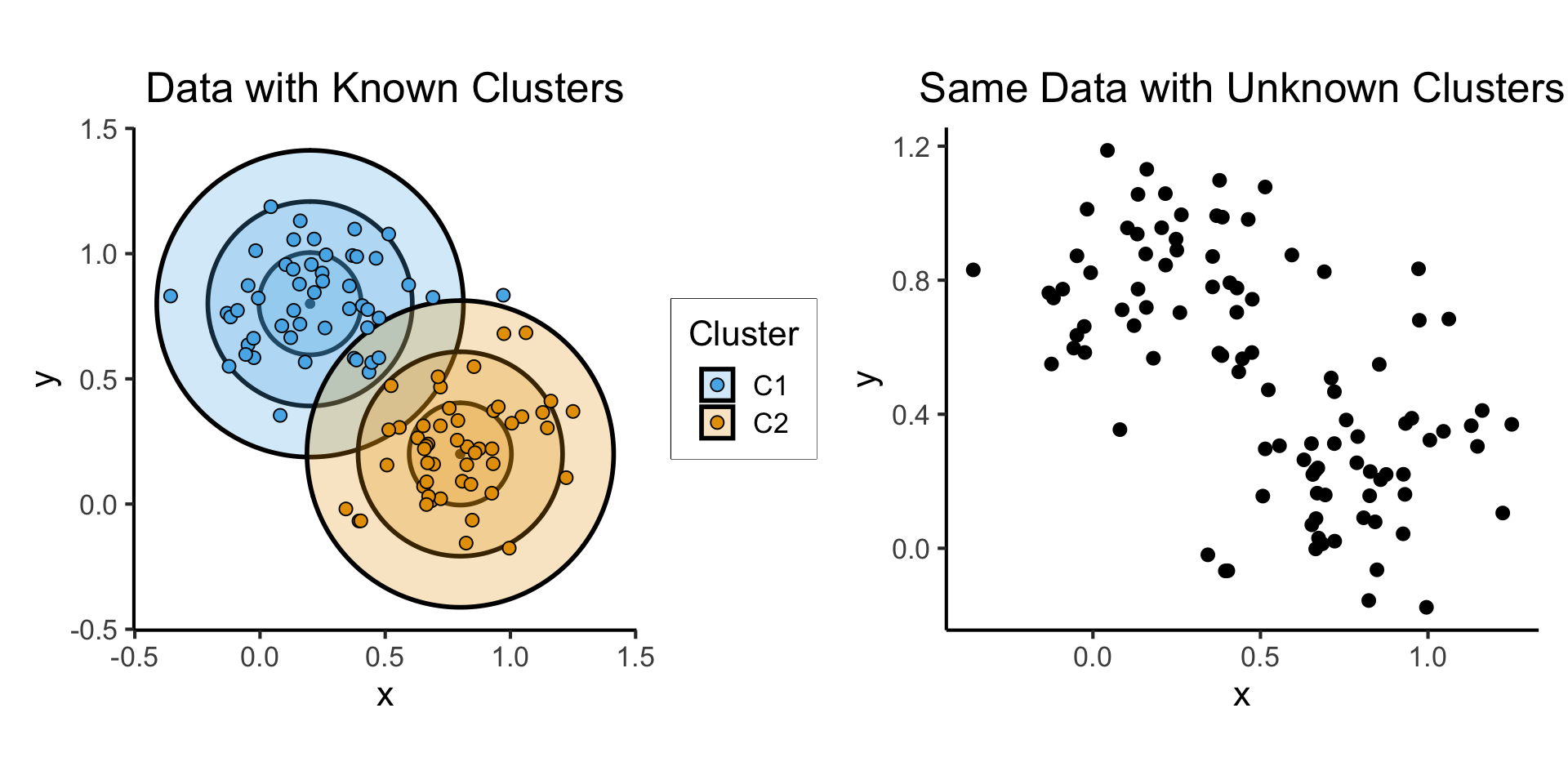
Clusters as Latent Variables
- Recall the Hidden Markov Model (one of many examples):
Modeling the Latent Distribution
- This observed/latent distinction gives us a modeling framework for inferring “underlying” distributions from data!
- Let’s begin with an overly-simple model: only one cluster (all data drawn from a single normal distribution)
Probability that RV \(X_i\) takes on value \(\mathbf{v}\):
\[ \begin{align*} &\Pr(X_i = \mathbf{v} \mid \param{\boldsymbol\theta_\mathcal{D}}) = \varphi_2(\mathbf{v}; \param{\boldsymbol\mu}, \param{\mathbf{\Sigma}}) \end{align*} \]
where \(\varphi_2(\mathbf{v}; \boldsymbol\mu, \mathbf{\Sigma})\) is pdf of \(\boldsymbol{\mathcal{N}}_2(\boldsymbol\mu, \mathbf{\Sigma})\).
Let \(\mathbf{X} = (X_1, \ldots, X_N)\), \(\mathbf{V} = (\mathbf{v}_1, \ldots, \mathbf{v}_N)\)
Probability that RV \(\mathbf{X}\) takes on values \(\mathbf{V}\):
\[ \begin{align*} &\Pr(\mathbf{X} = \mathbf{V} \mid \param{\boldsymbol\theta_\mathcal{D}}) \\ &= \Pr(X_1 = \mathbf{v}_1 \mid \paramDist) \times \cdots \times \Pr(X_N = \mathbf{v}_N \mid \paramDist) \end{align*} \]
So How Do We Infer Latent Vars From Data?
If only we had some sort of method for estimating which values of our unknown parameters \(\paramDist\) are most likely to produce our observed data \(\mathbf{X}\)
![]()
The diagram on the previous slide gave us an equation
\[ \begin{align*} \Pr(\mathbf{X} = \mathbf{V} \mid \param{\boldsymbol\theta_\mathcal{D}}) = \Pr(X_1 = \mathbf{v}_1 \mid \paramDist) \times \cdots \times \Pr(X_N = \mathbf{v}_N \mid \paramDist) \end{align*} \]
And we know that, when we consider the data as given and view this probability as a function of the parameters, we write it as
\[ \begin{align*} \lik(\mathbf{X} = \mathbf{V} \mid \param{\boldsymbol\theta_\mathcal{D}}) = \lik(X_1 = \mathbf{v}_1 \mid \paramDist) \times \cdots \times \lik(X_N = \mathbf{v}_N \mid \paramDist) \end{align*} \]
We want to find the most likely \(\paramDist\), that is, \(\boldsymbol\theta^*_\mathcal{D} = \argmax_{\paramDist}\mathcal{L}(\mathbf{X} = \mathbf{V} \mid \paramDist)\)
This value \(\boldsymbol\theta^*_\mathcal{D}\) is called the Maximum Likelihood Estimate of \(\paramDist\), and is easy to find using calculus tricks1
Handling Multiple Clusters
Probability \(X_i\) takes on value \(\mathbf{v}\):
\[ \begin{align*} &\Pr(X_i = \mathbf{v} \mid \param{C_i} = c_i; \; \param{\boldsymbol\theta_\mathcal{D}}) \\ &= \begin{cases} \varphi_2(v; \param{\boldsymbol\mu_1}, \param{\mathbf{\Sigma}}) &\text{if }c_i = 1 \\ \varphi_2(v; \param{\boldsymbol\mu_2}, \param{\mathbf{\Sigma}}) &\text{otherwise,} \end{cases} \end{align*} \]
where \(\varphi_2(v; \boldsymbol\mu, \mathbf{\Sigma})\) is pdf of \(\boldsymbol{\mathcal{N}}_2(\boldsymbol\mu, \mathbf{\Sigma})\).
Let \(\mathbf{C} = (\underbrace{C_1}_{\text{RV}}, \ldots, C_N)\), \(\mathbf{c} = (\underbrace{c_1}_{\mathclap{\text{scalar}}}, \ldots, c_N)\)
- Probability that RV \(\mathbf{X}\) takes on values \(\mathbf{V}\):
\[ \begin{align*} &\Pr(\mathbf{X} = \mathbf{V} \mid \param{\mathbf{C}} = \mathbf{c}; \; \param{\boldsymbol\theta_\mathcal{D}}) \\ &= \Pr(X_1 = \mathbf{v}_1 \mid \param{C_1} = c_1; \; \paramDist) \times \cdots \times \Pr(X_N = \mathbf{v}_N \mid \param{C_N} = c_N; \; \paramDist) \end{align*} \]
- It’s the same math as before! Find \((\mathbf{C}^*, \boldsymbol\theta^*_\mathcal{D}) = \argmax_{\param{\mathbf{C}}, \, \paramDist}\mathcal{L}(\mathbf{X} = \mathbf{V} \mid \param{\mathbf{C}}; \; \param{\boldsymbol\theta_\mathcal{D}})\)
Dimensionality Reduction (W10)
- High-level goal: Retain information about word-context relationships while reducing the \(M\)-dimensional representations of each word down to 3 dimensions.
- Low-level goal: Generate rank-\(K\) matrix \(\mathbf{W}\) which best approximates distances between words in \(M\)-dimensional space (rows in \(\mathbf{X}\))
Looking Forward
Backing Up: What is a Neural Network?
- A linked network of \(L\) layers each containing nodes \(\nu_i^{[\ell]}\)
What Do the Nodes Do?
Each node \(\nu_i^{[\ell]}\) in the network:
- Takes in an input,
- Transforms it using a weight \(w^{[\ell]}_i\) and bias \(b^{[\ell]}_i\), and
- Produces an output, typically using a sigmoid function like \(\sigma(x) = \frac{1}{1+e^{-x}}\):
\[ \text{output}^{[\ell]}_i = \sigma(w^{[\ell]}_i \cdot \text{input} + b^{[\ell]}_i) \]
How Does it “Learn”?
- Need a loss function \(\mathcal{L}(\widehat{y}, y)\)
- Starting from the end, we backpropagate the loss, updating weights and biases as we go
- Higher loss \(\implies\) greater change to weights and biases
Core Courses
- DSAN 5200: Advanced Data Visualization
- DSAN 5300: Statistical Learning
- (DSAN 6000: Big Data and Cloud Computing)
Elective Courses
- DSAN 5500: Data Structures, Objects, and Algorithms in Python
- (DSAN 5700: Blockchain Technologies)
- DSAN 6800: Principles of Cybersecurity
- DSAN 6500: Comp Vision and Generative Image Modeling
- DSAN 6550: Adaptive Measurement
- DSAN 6600: Neural Nets & Deep Learning
- DSAN 6650: Reinforcement Learning
- DSAN 5600: Applied Time Series for Data Science
- (DSAN 6200: Analytics and Math for Streaming and High Dimension Data)
- DSAN 5400: Comp Ling, Advanced Python
- (DSAN 5810: NLP with Large Language Models)
- DSAN 5450: Data Ethics and Policy
- (DSAN 5550: Data Science and Climate Change)
- DSAN 5900: Digital Storytelling
Types of Data
- DSAN 5600: Applied Time Series for Data Science
- DSAN 5400: Computational Linguistics, Advanced Python
- (DSAN 5810: NLP with Large Language Models)
- DSAN 6550: Adaptive Measurement
- (DSAN 5550: Data Science and Climate Change)
- (DSAN 6750: GIS for Spatial Data Science)
- DSAN 6500: Comp Vision and Generative Image Modeling
- DSAN 5500: Data Structures
- DSAN 5900: Digital Storytelling
Future Electives!
- DSAN 6100: Optimization
- DSAN 6300: Database Systems and SQL
- DSAN 6400: Network Analytics [Summer]
- DSAN 6700: Machine Learning App Deployment
- DSAN 6750: GIS for Spatial Data Science
- DSAN 6850: Causal Inference for Computational Social Science [Summer]
References
DSAN 5000 W13: Course Wrapup