Week 7: Spatial Data Science: Three Forms of Spatial Autocorrelation

PPOL 6805 / DSAN 6750: GIS for Spatial Data Science
Fall 2025

Author

Affiliation

Jeff Jacobs

jj1088@georgetown.edu

Open slides in new tab →

Random Fields

\[ \text{Data} = \left\{Z(\mathbf{s}) \mid \mathbf{s} \in D \subset \mathbb{R}^2\right\} \]

\(D\) = Rectangle; \(Z(\mathbf{s})\) here: height at coordinate \(\mathbf{s} \in D\)

Key Notation / Definition

2-Dimensional Spatial Process (Schabenberger and Gotway 2004, 6)

\[ \text{Data} = \left\{Z(\mathbf{s}) \mid \mathbf{s} \in D \subset \mathbb{R}^d\right\} \]

	Geostatistical Data	Lattice/Region Data	Point Pattern
Criteria	Fixed \(D\), Continuous	Fixed \(D\), Discrete	Random subset \(D^* \subseteq D\)
What's Random?	Value of \(Z\) at POINT \(\mathbf{s}_i \in D\)	Value of \(Z\) across POLYGON \(\mathbf{r}_i \subseteq D\)	Subset \(D^*\) formed by events
Interest	Infer non-observed parts of \(D\)	Autocorrelation, clustering	Point-generating process
Example	Dumping sand on a table \(D = \{(x,y) \mid x \in [0,2], y \in [0,1]\}\) \(Z(\mathbf{s}_i)\): Attribute(s) at site \(\mathbf{s}_i\) (at coordinate \(\mathbf{s}_i = (x_i,y_i)\)) Example: Height of sand. \(Z(\mathbf{s}_1) = 500\text{m}\), \(Z(\mathbf{s}_2) = 850\text{m}\), \(\ldots\)	\(Z(\mathbf{s})\) observed over \(N \times N\) grid of plots Well-defined ‘Neighbors’ (next section!) Autocorrelation: Are points around \(\mathbf{s}_i\) likely to have values similar to \(Z(\mathbf{s}_i)\)?	Unknown number of lightning strikes \(\mathbf{s}_1, \mathbf{s}_2, \ldots\) All of \(D\) is observed, but what determines subset \(D^*\) where events occur? Unmarked: Locations only Marked: Locations+info (e.g., intensity of strike)

Geostatistical Data: Dumping Sand onto a Table!

• Domain \(D\): tabletop; Random process: dumping sand onto the tabletop
• \(\Omega\): All possible realizations of process. \(\omega_i \in \Omega\) Particular realization

Figure 1: \(\omega_1 \in \Omega\)

Figure 2: \(\omega_2 \in \Omega\)

Figure 3: \(\omega_3 \in \Omega\)

Figure 4: \(\omega_4 \in \Omega\)

Example: Water Coverage in Bhola, Bangladesh

ArcGIS: Sea Level Rise in Bangladesh (See also)

Parenti (2011)

Geostatistical Modeling: Terrains Are Not Spiky Chaotic Landscapes!

Geostatistical Data \(\rightarrow\) Point Pattern

• Indicator function: \(\mathbb{1}\left[Z(\mathbf{s}) > 860\text{m}\right]\)

set.seed(6805)
library(tidyverse)

── Attaching core tidyverse packages ──────────────────────── tidyverse 2.0.0 ──
✔ dplyr     1.1.4     ✔ readr     2.1.5
✔ forcats   1.0.0     ✔ stringr   1.5.1
✔ ggplot2   3.5.1     ✔ tibble    3.3.0
✔ lubridate 1.9.4     ✔ tidyr     1.3.1
✔ purrr     1.0.4     
── Conflicts ────────────────────────────────────────── tidyverse_conflicts() ──
✖ dplyr::filter() masks stats::filter()
✖ dplyr::lag()    masks stats::lag()
ℹ Use the conflicted package (<http://conflicted.r-lib.org/>) to force all conflicts to become errors

library(sf)

Linking to GEOS 3.11.0, GDAL 3.5.3, PROJ 9.1.0; sf_use_s2() is TRUE

library(terra)

terra 1.8.60

Attaching package: 'terra'

The following object is masked from 'package:tidyr':

    extract

library(latex2exp)
#### Define area
lat_range <- c(-5.0, -6.0)
lon_range <- c(15, 20)
#lon_center <- -5.4
#lat_center <- 36.75
# And the window around this centroid
lat_radius <- 0.05
lon_radius <- 0.1

gen_random_table <- function(world_num=1, return_data=FALSE, rand_seed=NULL) {
  if (!is.null(rand_seed)) {
    set.seed(rand_seed)
  } else {
    rand_seed <- sample(1:9999, size=1)
    set.seed(rand_seed)
  }
  lat_center <- runif(1, min=min(lat_range), max=max(lat_range))
  lon_center <- runif(1, min=min(lon_range), max=max(lon_range))
  lon_lower <- lon_center - lon_radius
  lon_upper <- lon_center + lon_radius
  lat_lower <- lat_center - lat_radius
  lat_upper <- lat_center + lat_radius
  coords <- data.frame(x = c(lon_lower, lon_lower, lon_upper, lon_upper),
                       y = c(lat_lower, lat_upper, lat_lower, lat_upper))
  coords_sf <- st_as_sf(coords, coords = c("x", "y"), crs = 4326)
  # Using geodata
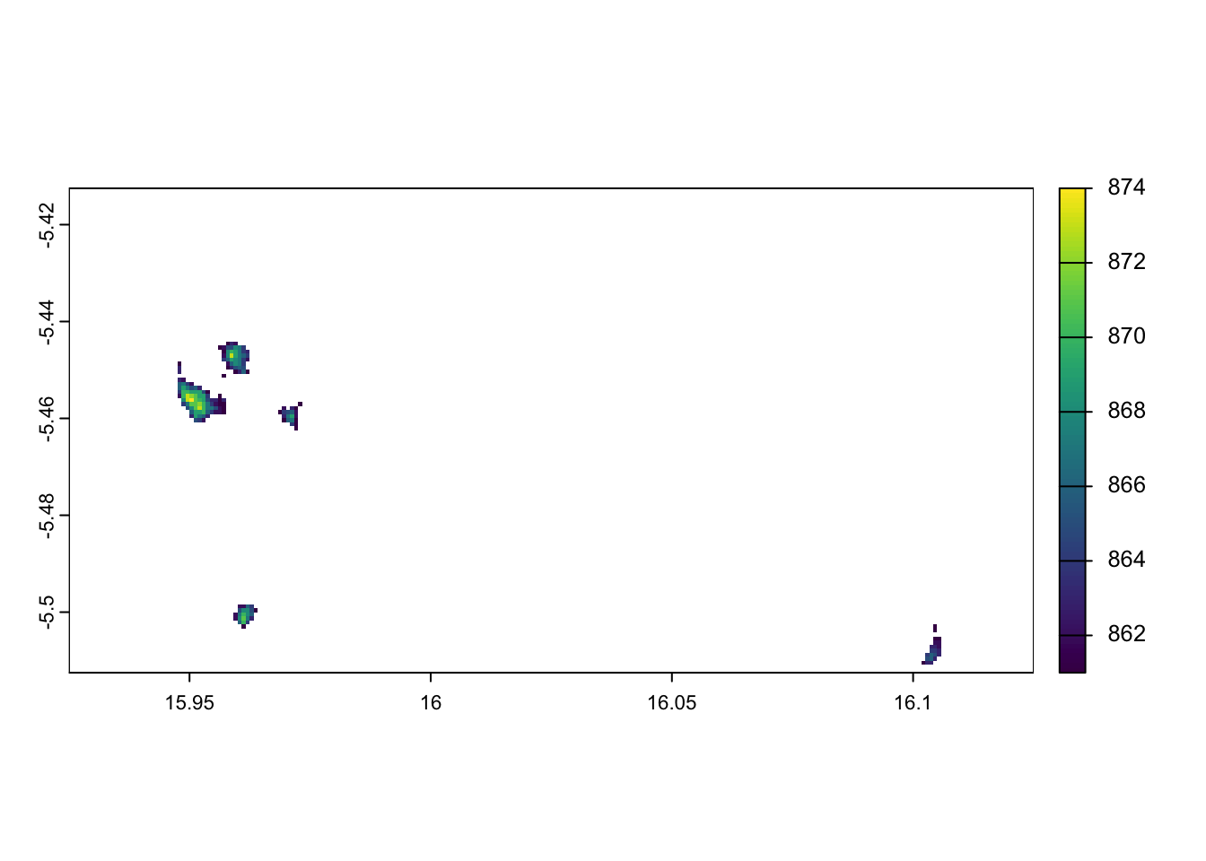
  elev <- geodata::elevation_3s(lon = lon_center, lat = lat_center, res=2.5, path = getwd())
  elev <- terra::crop(elev, coords_sf)
  return(elev)
}

compute_hillshade <- function(elev) {
  # Calculate hillshade
  slopes <- terra::terrain(elev, "slope", unit = "radians")
  aspect <- terra::terrain(elev, "aspect", unit = "radians")
  hs <- terra::shade(slopes, aspect)
  return(hs)
}

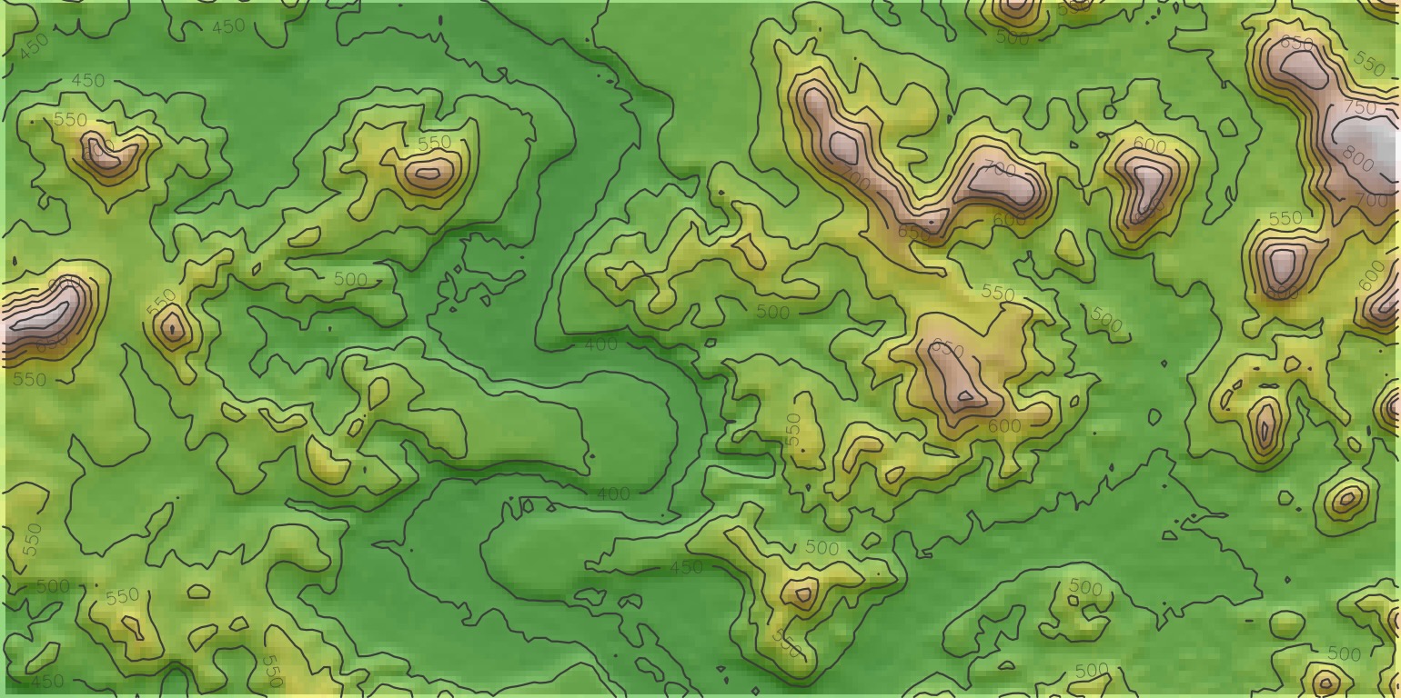
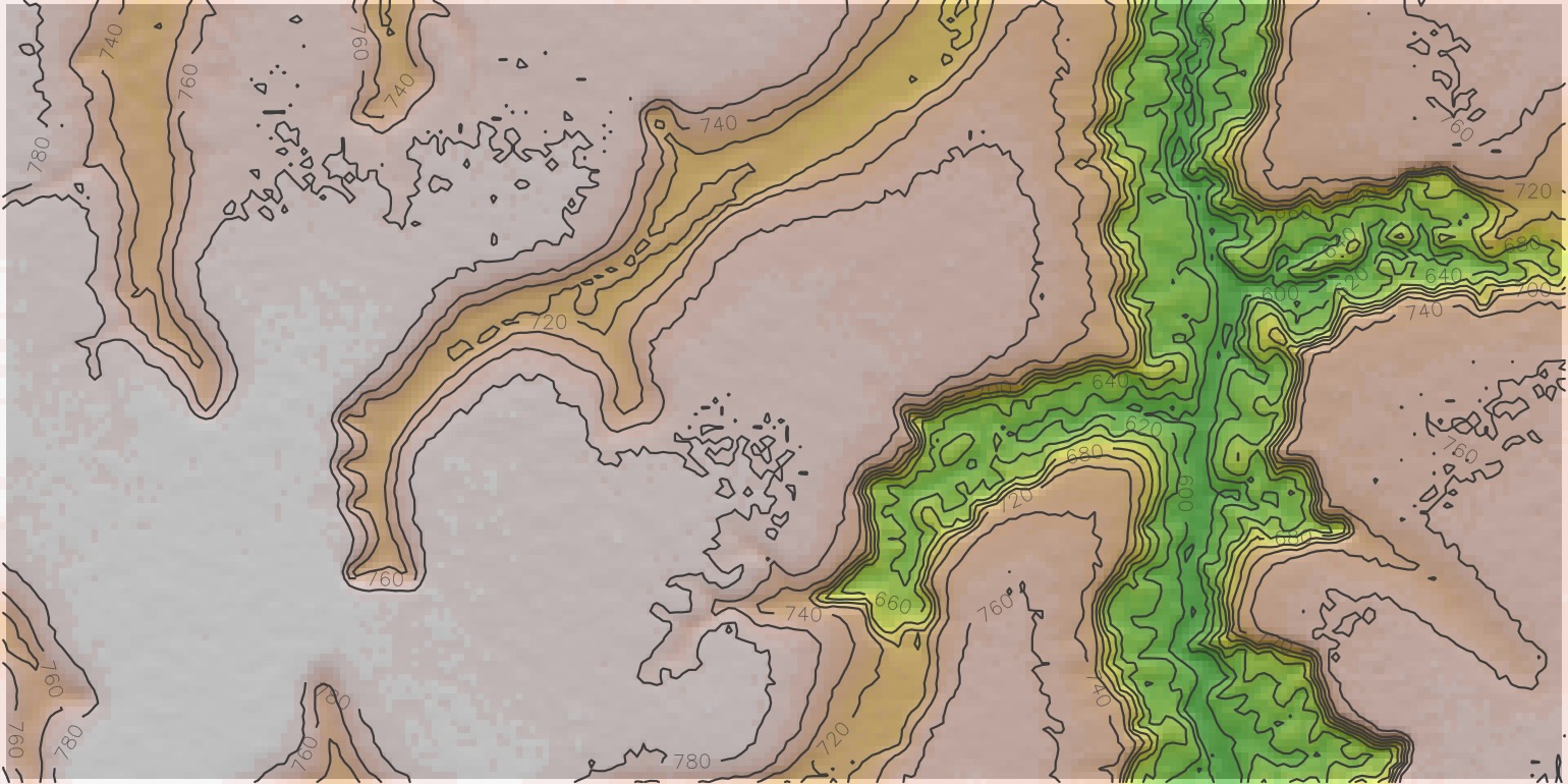
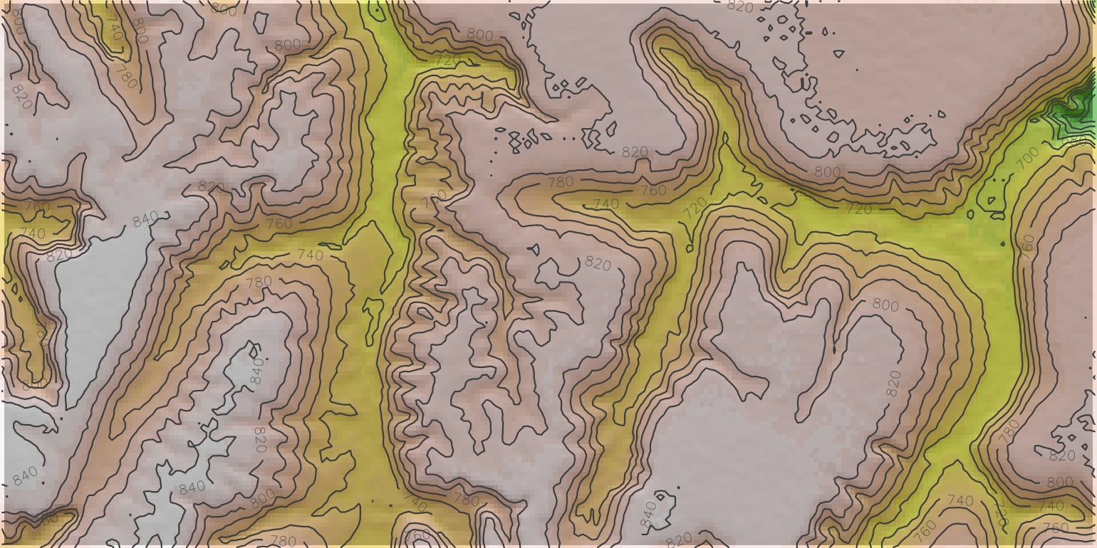
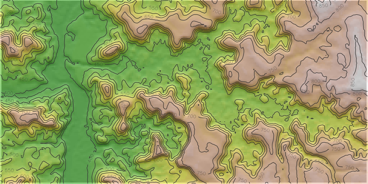
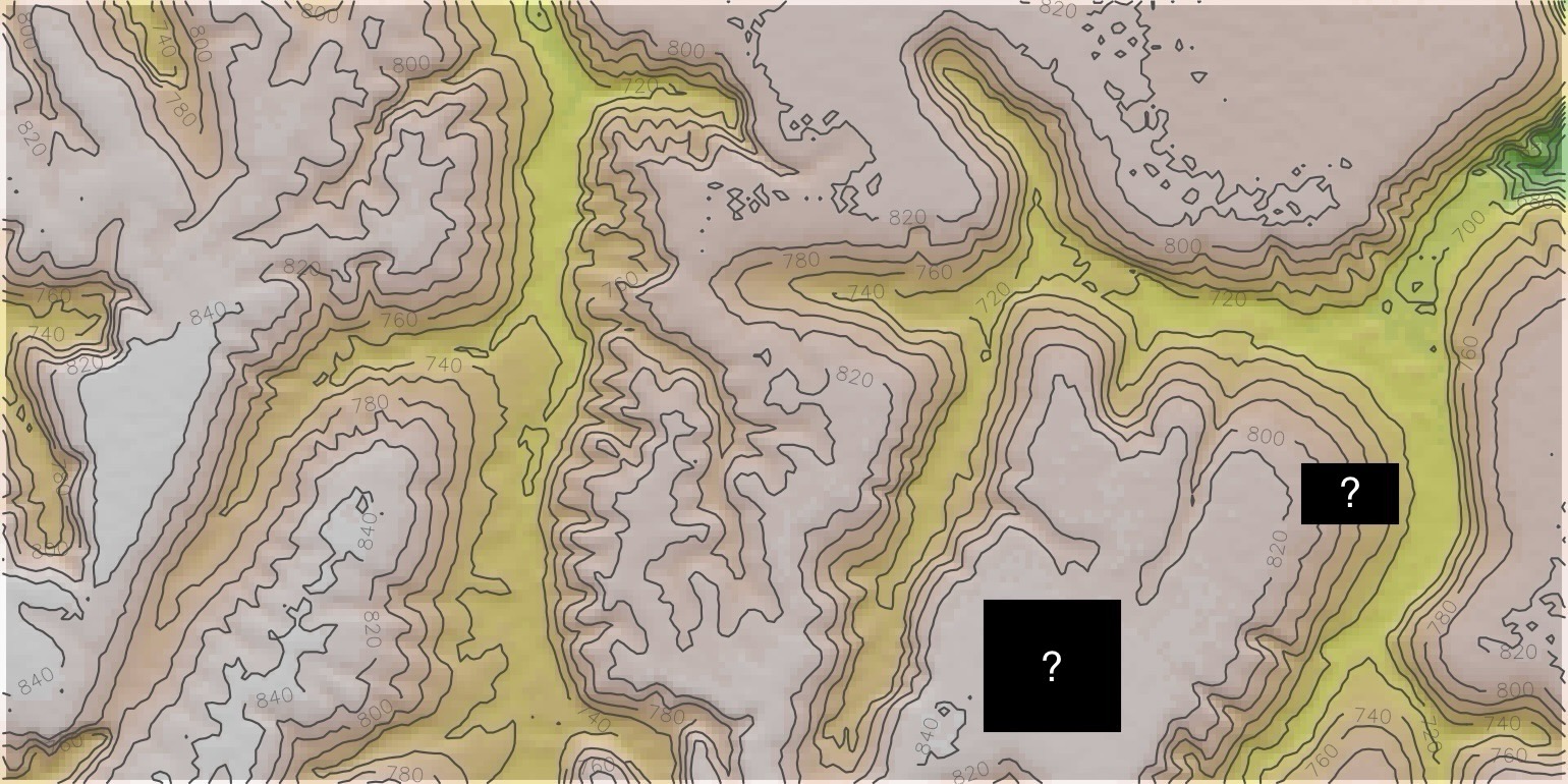
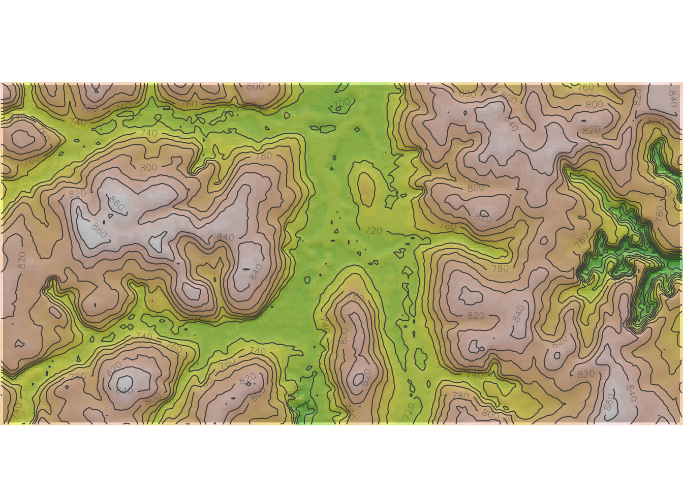
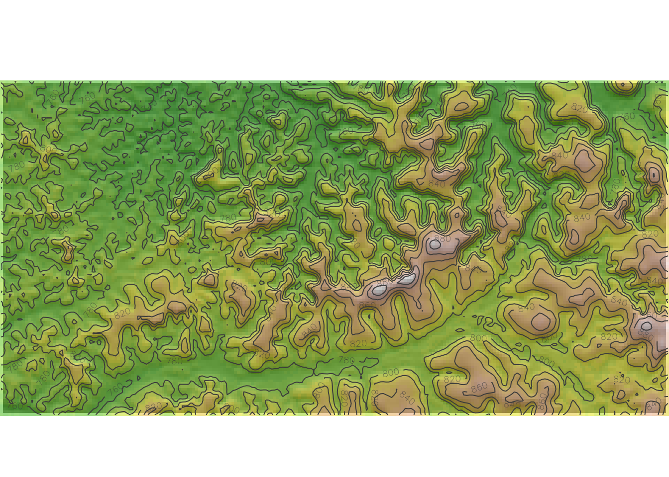
plot_hillshade <- function(elev, hs, title=NULL) {
  ## Plot hillshading as basemap
  # (here using terra::plot, but could use tmap)
  # lat_upper_trimmed <- lat_upper - 0.001*lat_upper
  # lat_lower_trimmed <- lat_lower - 0.001*lat_lower
  base_plot <- terra::plot(
    hs, col = gray(0:100 / 100), legend = FALSE, axes = FALSE, mar=c(0,0,1,0), grid=TRUE
  )
  #    xlim = c(elev_xmin, elev_xmax), ylim = c(elev_ymin, elev_ymax))
  # overlay with elevation
  
  color_vec <- terrain.colors(25)
  plot(elev, col = color_vec, alpha = 0.5, legend = FALSE, axes = FALSE, add = TRUE)
  
  # add contour lines
  terra::contour(elev, col = "grey30", add = TRUE)
  if (!is.null(title)) {
    world_name <- TeX(sprintf(r"(World $\omega_{%d} \in \Omega$)", world_num))
    title(world_name)
  }
}
elev_r1 <- gen_random_table(rand_seed=6810)
hs_r1 <- compute_hillshade(elev_r1)
plot_hillshade(elev_r1, hs_r1)

terra::ifel(
  elev_r1 > 860, elev_r1, NA
) |> plot()

elev_r2 <- gen_random_table(rand_seed=6815)
hs_r2 <- compute_hillshade(elev_r2)
plot_hillshade(elev_r2, hs_r2)

my_quant <- function(x) quantile(x, 0.99)
elev_99 <- terra::global(elev_r2, my_quant)[1,1]
elev_indic_r2 <- terra::ifel(
  elev_r2 > elev_99, elev_r2, NA
)
plot(elev_indic_r2)

Geospatial Data \(\rightarrow\) Lattice/Region Data

table_elev <- gen_random_table(rand_seed=6805)
table_hs <- compute_hillshade(table_elev)
#plot_hillshade(table_elev, table_hs)
#par(mfrow=c(1,2), mar=c(0,0,1,1))
plot(table_elev)

(Pretend this is infinite-resolution) Infinite number of neighbors around each point!

elev_coarse <- terra::aggregate(table_elev, 12)
plot(elev_coarse)

Finite number of neighbors around each observation \(\implies\) Can study correlations between neighboring cells!

Doing Things with nbdep

• “Neighbor” Definitions
• Testing Hypotheses About Neighborhoods!

Who Are My Neighbors?

• Contiguity-Based:

• Distance-Based

• \(K\)-Nearest Neighbors

Distance-Based Neighbors

From Xie (2022)

Spatial Autocorrelation

• Location \(i\) has high value \(\implies\) locations near \(i\) more likely to have high values

Moran’s \(I\)

\[ I = \underset{\text{Inverse of Variance}}{\boxed{\frac{n}{\sum_{i=1}^{n}(y_i - \overline{y})^2}}} \frac {\overbrace{\sum_{i=1}^{n}\sum_{j=1}^{n}w_{ij}(y_i - \overline{y})(y_j - \overline{y})}^{\text{Weighted Covariance}}} {\underbrace{\sum_{i=1}^{n}\sum_{j=1}^{n}w_{ij}}_{\text{Normalize Weights}}} \]

• \(I\) is Large when:
  • \(y_i\) and \(y_j\) are neighbors: \(w_{ij}\), and
  • \(y_i\) and \(y_j\) large at the same time: \((y_i - \overline{y})(y_j - \overline{y})\)

Local Indicators of Spatial Autocorrelation (LISA)

• tldr: See how much a given location \(\mathbf{s}\) contributes to overall Moran’s \(I\)
• Local Moran’s \(I\):

\[ I_i = \frac{y_i - \overline{y}}{S_i^2}\sum_{j=1}^{n}w_{ij}(y_j - \overline{y}) \]

References

Parenti, Christian. 2011. Tropic of Chaos: Climate Change and the New Geography of Violence. PublicAffairs.

Schabenberger, Oliver, and Carol A. Gotway. 2004. Statistical Methods for Spatial Data Analysis. CRC Press.

Xie, Sherrie. 2022. “Analyzing Geospatial Data in R.” R/Medicine Virtual Conference: YouTube.