library(tidyverse)
library(spatstat)
set.seed(6805)
N <- 60
r_core <- 0.05
obs_window <- square(1)
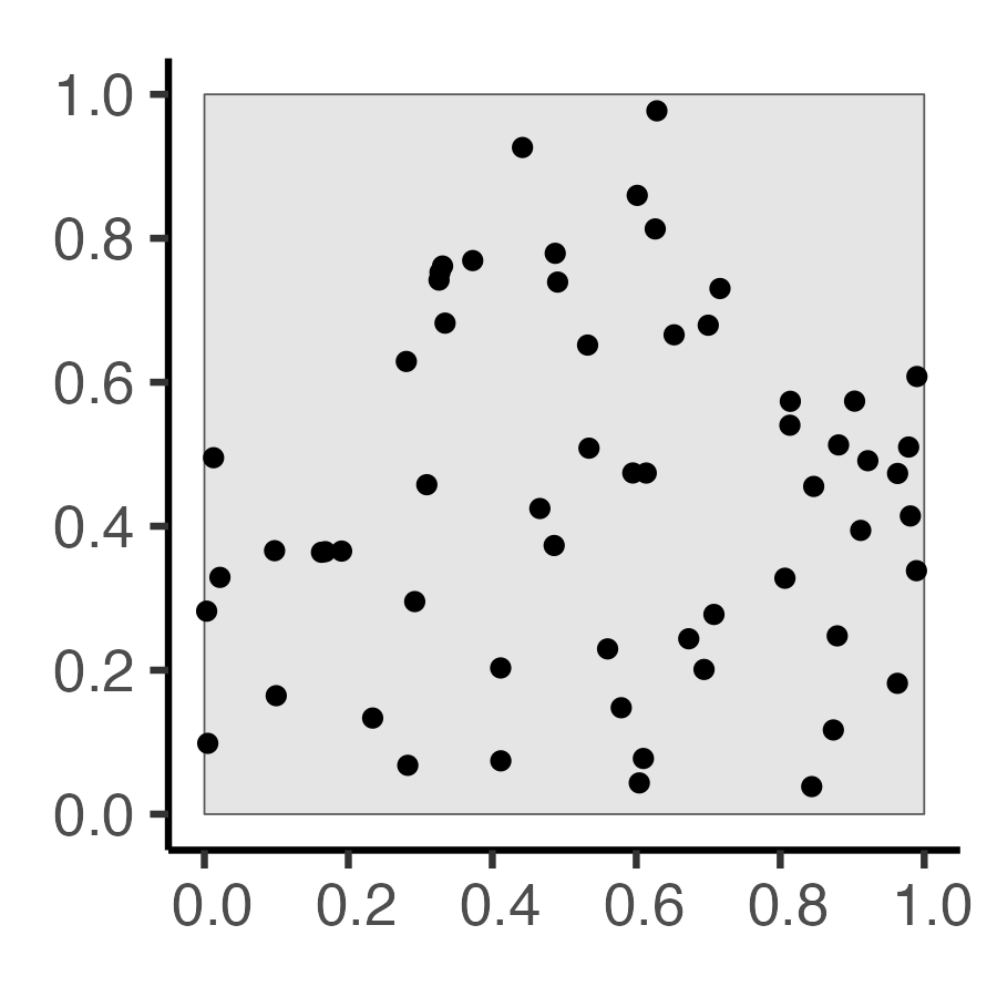
# Regularity via Inhibition
#reg_sims <- rMaternI(N, r=r_core, win=obs_window)
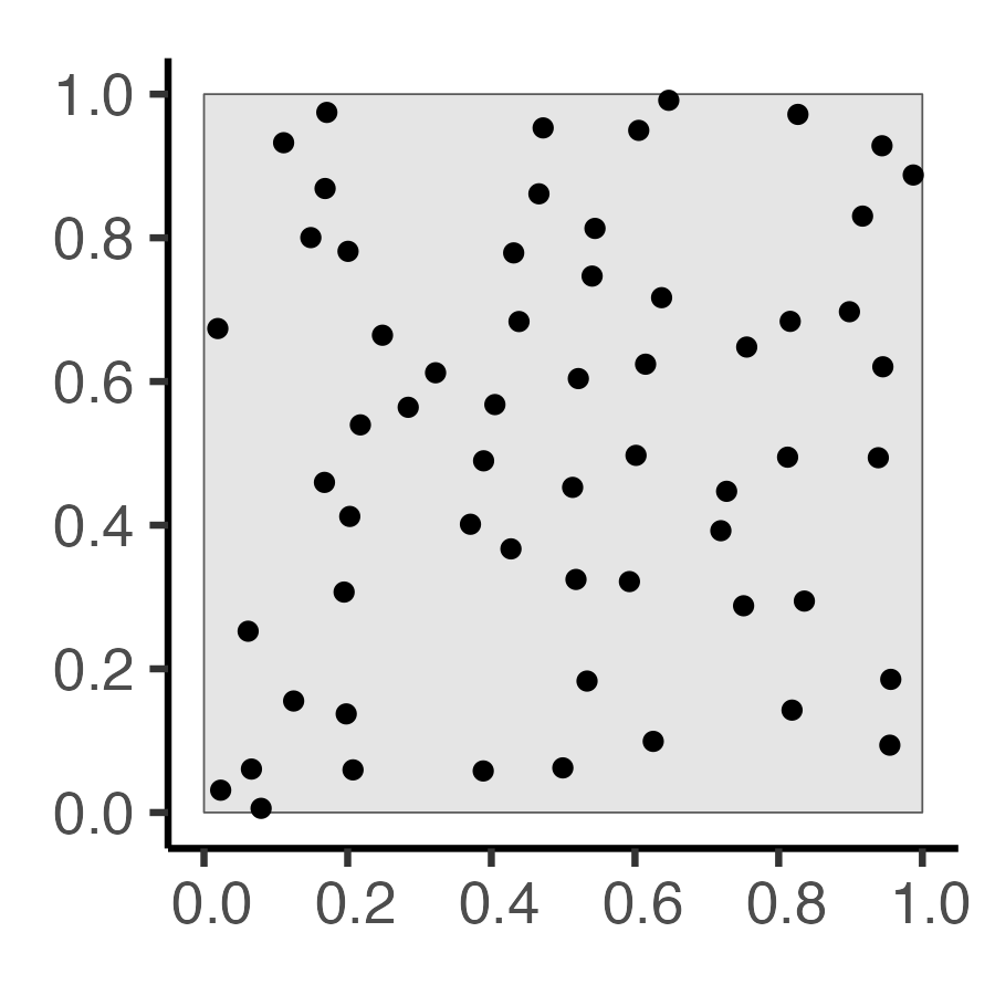
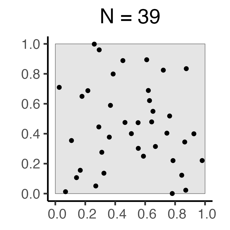
cond_reg_sims <- rSSI(r=r_core, N)
# CSR data
#csr_sims <- rpoispp(N, win=obs_window)
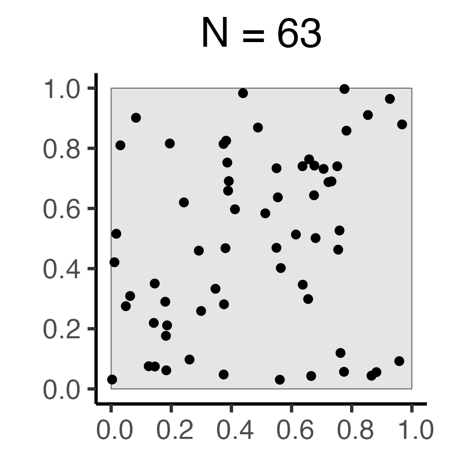
cond_sr_sims <- rpoint(N, win=obs_window)
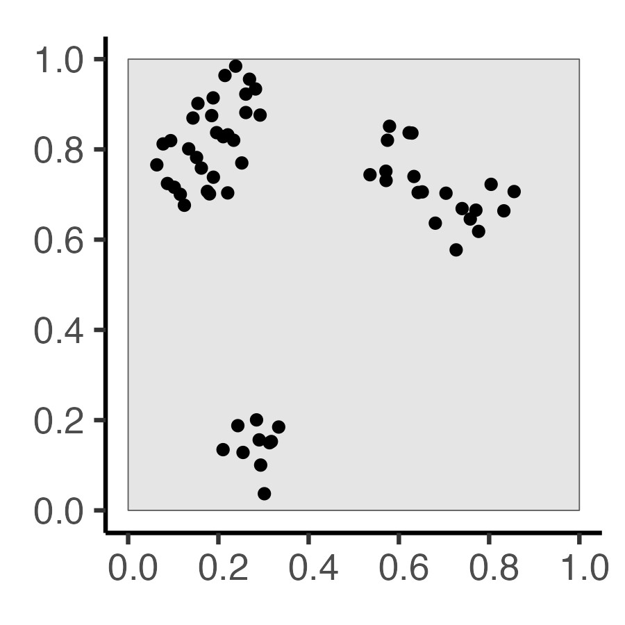
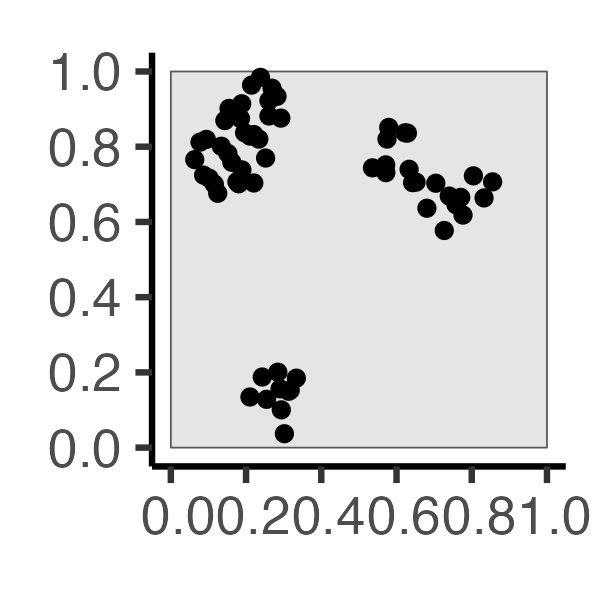
### Clustered data
#clust_sims <- rMatClust(kappa=6, r=2.5*r_core, mu=10, win=obs_window)
#clust_sims <- rMatClust(mu=5, kappa=1, scale=0.1, win=obs_window, n.cond=N, w.cond=obs_window)
#clust_sims <- rclusterBKBC(clusters="MatClust", kappa=10, mu=10, scale=0.05, verbose=FALSE)
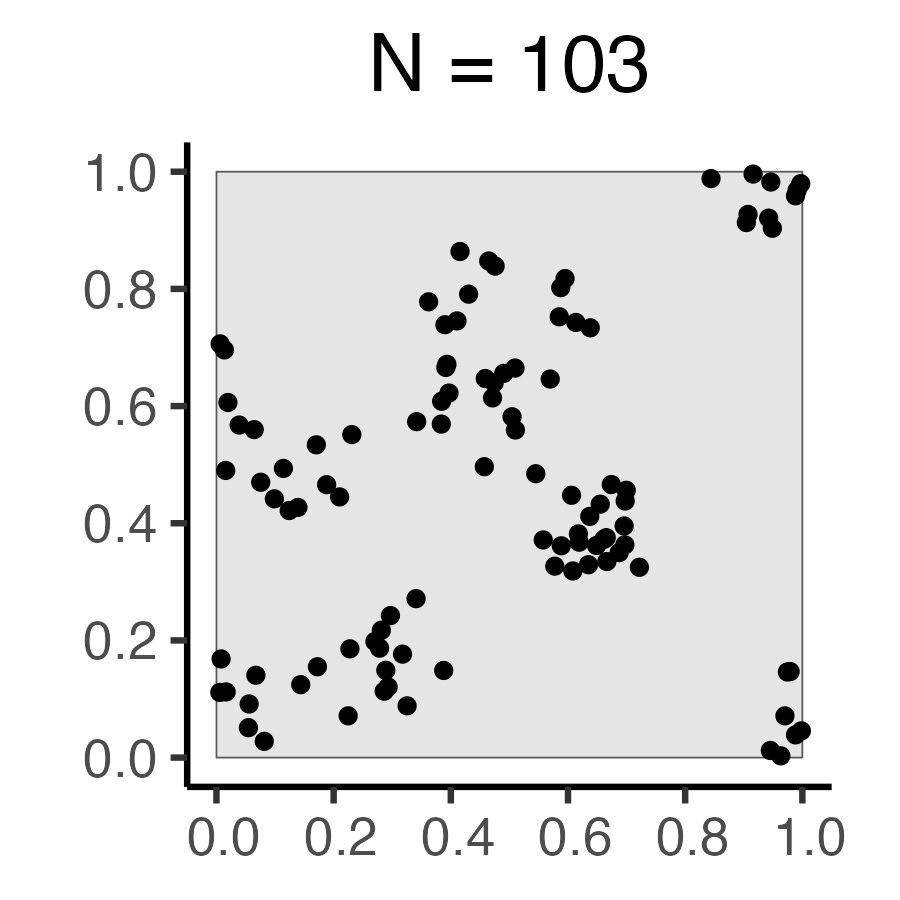
# Each cluster consist of 10 points in a disc of radius 0.2
nclust <- function(x0, y0, radius, n) {
#print(n)
return(runifdisc(10, radius, centre=c(x0, y0)))
}
cond_clust_sims <- rNeymanScott(kappa=5, expand=0.0, rclust=nclust, radius=2*r_core, n=10)
# And PLOT
plot_w <- 400
plot_h <- 400
plot_scale <- 2.25
cond_reg_plot <- cond_reg_sims |> sf::st_as_sf() |>
ggplot() +
geom_sf() +
dsan_theme()
ggsave("images/cond_reg.png", cond_reg_plot, width=plot_w, height=plot_h, units="px", scale=plot_scale)
cond_sr_plot <- cond_sr_sims |> sf::st_as_sf() |>
ggplot() +
geom_sf() +
dsan_theme()
ggsave("images/cond_sr.png", cond_sr_plot, width=plot_w, height=plot_h, units="px", scale=plot_scale)
cond_clust_plot <- cond_clust_sims |> sf::st_as_sf() |>
ggplot() +
geom_sf() +
dsan_theme()
ggsave("images/cond_clust.png", cond_clust_plot, width=plot_w, height=plot_h, units="px", scale=plot_scale)