Week 2: How Do Maps Work?

PPOL 6805 / DSAN 6750: GIS for Spatial Data Science
Fall 2025

Author

Affiliation

Jeff Jacobs

jj1088@georgetown.edu

Open slides in new tab →

Schedule

Today’s Planned Schedule:

	Start	End	Topic
Lecture	6:30pm	6:50pm	Logistics 1: JupyterHub x Positron →
	6:50pm	7:15pm	Logistics 2: Reducing Fear →
	7:20pm	7:50pm	Building Our First Map! →
Break!	7:50pm	8:00pm
	8:00pm	8:30pm	Raster Data →
	8:30pm	9:00pm	Finding GIS Data →

source("../dsan-globals/_globals.r")
set.seed(5300)

\[ \DeclareMathOperator*{\argmax}{argmax} \DeclareMathOperator*{\argmin}{argmin} \newcommand{\bigexp}[1]{\exp\mkern-4mu\left[ #1 \right]} \newcommand{\bigexpect}[1]{\mathbb{E}\mkern-4mu \left[ #1 \right]} \newcommand{\definedas}{\overset{\small\text{def}}{=}} \newcommand{\definedalign}{\overset{\phantom{\text{defn}}}{=}} \newcommand{\eqeventual}{\overset{\text{eventually}}{=}} \newcommand{\Err}{\text{Err}} \newcommand{\expect}[1]{\mathbb{E}[#1]} \newcommand{\expectsq}[1]{\mathbb{E}^2[#1]} \newcommand{\fw}[1]{\texttt{#1}} \newcommand{\given}{\mid} \newcommand{\green}[1]{\color{green}{#1}} \newcommand{\heads}{\outcome{heads}} \newcommand{\iid}{\overset{\text{\small{iid}}}{\sim}} \newcommand{\lik}{\mathcal{L}} \newcommand{\loglik}{\ell} \DeclareMathOperator*{\maximize}{maximize} \DeclareMathOperator*{\minimize}{minimize} \newcommand{\mle}{\textsf{ML}} \newcommand{\nimplies}{\;\not\!\!\!\!\implies} \newcommand{\orange}[1]{\color{orange}{#1}} \newcommand{\outcome}[1]{\textsf{#1}} \newcommand{\param}[1]{{\color{purple} #1}} \newcommand{\pgsamplespace}{\{\green{1},\green{2},\green{3},\purp{4},\purp{5},\purp{6}\}} \newcommand{\pedge}[2]{\require{enclose}\enclose{circle}{~{#1}~} \rightarrow \; \enclose{circle}{\kern.01em {#2}~\kern.01em}} \newcommand{\pnode}[1]{\require{enclose}\enclose{circle}{\kern.1em {#1} \kern.1em}} \newcommand{\ponode}[1]{\require{enclose}\enclose{box}[background=lightgray]{{#1}}} \newcommand{\pnodesp}[1]{\require{enclose}\enclose{circle}{~{#1}~}} \newcommand{\purp}[1]{\color{purple}{#1}} \newcommand{\sign}{\text{Sign}} \newcommand{\spacecap}{\; \cap \;} \newcommand{\spacewedge}{\; \wedge \;} \newcommand{\tails}{\outcome{tails}} \newcommand{\Var}[1]{\text{Var}[#1]} \newcommand{\bigVar}[1]{\text{Var}\mkern-4mu \left[ #1 \right]} \]

Logistics 1: JupyterHub x Positron

Logistics 2: Reducing Fear 💆

• Jeff’s Post-Week 1 自我革命
• Weekly Coding Workshops
• How To Not Be Scared of Prerequisites
• ChatGPT
• Learning How To Learn

Top secret translation for me: zi4 wo2 ge1 ming4

Helpful Feedback!

• Sry for machine-gunning words/concepts at you last week
  • \(\leadsto\) Talking more slowly!
  • \(\leadsto\) Less colloquial language!
  • Pls give me grace as I enact this video in reverse
• More importantly: weekly coding workshops!
  • Not only will they “cancel out” my too-fast DC-slang-poisoned pace, but also…
  • Focus will be on specific blocks of code rather than higher-level concepts [but see also: “forgetting curve” diagram a few slides ahead]

Pedagogical Principles

• There’s literally no such thing as “intelligence”
• Anyone is capable of learning anything (neural plasticity)
• Growth mindset: “I can’t do this” \(\leadsto\) “I can’t do this yet!”
• The point of a class is learning: understanding something about the world, either (a) For its own sake (end in itself) or (b) Because it’s relevant to something you care about (means to an end)

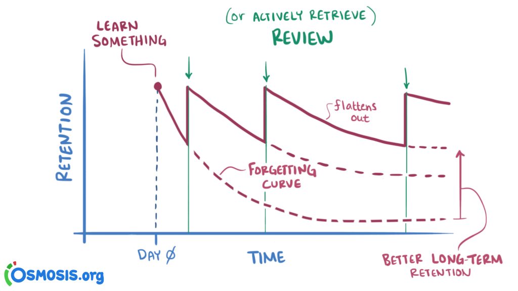
Our teaching should be governed, not by a desire to make students learn things, but by the endeavor to keep burning within them that light which is called curiosity. (Montessori 1916)

ChatGPT and Whatnot

• If you feel like ChatGPT will help you learn something in the course, then use it!
• If you feel like you’re using it as a “crutch”, try to hold yourself accountable for not using it!

Take the time/energy you're using to worry about...	Use it instead to worry about...
ChatGPT Collaboration Policies Plagiarism	Learning GIS

On Not Worrying About Prereqs

• I genuinely believe that I can make the course accessible to you, meeting you wherever you’re at, no matter what!
• Everyone learns at their own pace (who says 14 weeks is “correct” amount of time to learn GIS?), and I structure my courses as best as I possibly can to adapt to your pace
• \(\Rightarrow\) Assessments (HW, Midterm) valuable in two ways:
• [Valuable for you] As an accountability mechanism to make sure you’re learn the material (how do we know when we’ve learned something? When we can answer questions about it / use it to accomplish things!)
• [Valuable for me] For assessing and updating pace

R and/or Python and/or JS

• My Geometry vs. Algebra Rant… Euclid’s Elements, Book VI, Proposition 28.
• The problem: Divide a given straight line so that the rectangle contained by its segments may be equal to a given area, not exceeding the square of half the line.

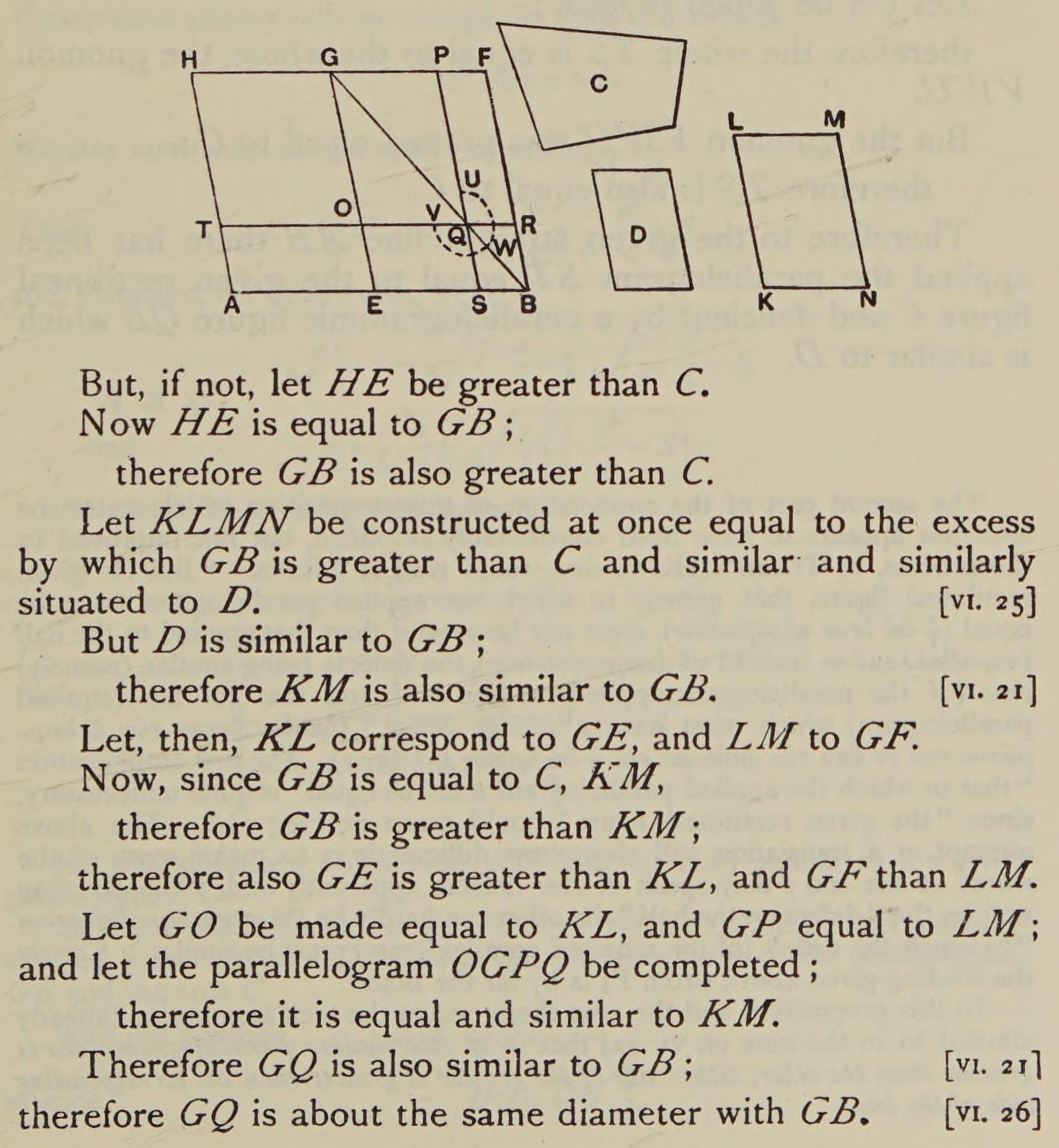
Geometers solved w/geometry (300 BC)…

…Algebraists solved w/algebra (2000 BC)…

\[ \begin{align*} &ax^2 + bx + c = 0 \\ \Rightarrow \; & x_+ = \frac{-b + \sqrt{b^2 - 4ac}}{2a} \end{align*} \]

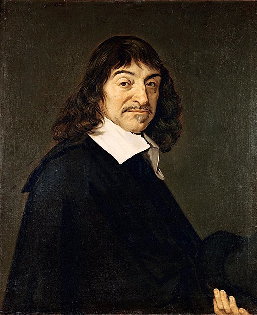
…From 1637 onwards, whichever is easier! 🤯🤯🤯 (Isomorphism)

Figure 1: Circle with radius 1? Or \((x,y)\) satisfying \(x^2 + y^2 = 1\)?

Learning How To Learn

Figure 2: From The Carter (Documentary)

He’s Literally Extremely Correct!

From Elsevier Osmosis: Spaced Repetition

Let’s Make Some Dang Maps!

Our First Map: Polygons!

(Quick demo adapted from Sherry Xie’s R Consortium Workshop: Analyzing Geospatial Data in R, using DC rather than Philadelphia open data.)

library(sf)
# Load DC tracts data
dc_sf_fpath <- "data/DC_Census_2020/Census_Tracts_in_2020.shp"
dc_sf <- st_read(dc_sf_fpath);

Reading layer `Census_Tracts_in_2020' from data source 
  `/Users/jpj/gtown-local/ppol6805/w02/data/DC_Census_2020/Census_Tracts_in_2020.shp' 
  using driver `ESRI Shapefile'
Simple feature collection with 206 features and 315 fields
Geometry type: POLYGON
Dimension:     XY
Bounding box:  xmin: -8584933 ymin: 4691871 xmax: -8561515 ymax: 4721078
Projected CRS: WGS 84 / Pseudo-Mercator

cols_to_keep <- c("OBJECTID", "TRACT", "GEOID", "ALAND", "AWATER", "STUSAB", "SUMLEV", "GEOCODE", "STATE", "NAME", "POP100", "HU100", "geometry")
dc_sf <- dc_sf |> select(cols_to_keep)

Warning: Using an external vector in selections was deprecated in tidyselect 1.1.0.
ℹ Please use `all_of()` or `any_of()` instead.
  # Was:
  data %>% select(cols_to_keep)

  # Now:
  data %>% select(all_of(cols_to_keep))

See <https://tidyselect.r-lib.org/reference/faq-external-vector.html>.

sf Objects

dc_sf is an object of type sf (short for “simple feature”), which extends data.frame, and contains features which have type POLYGON

class(dc_sf)

[1] "sf"         "data.frame"

head(dc_sf)

OBJECTID	TRACT	GEOID	ALAND	AWATER	STUSAB	SUMLEV	GEOCODE	STATE	NAME	POP100	HU100	geometry
1	002002	11001002002	849376	0	DC	140	11001002002	11	Census Tract 20.02	4072	1532	POLYGON ((-8575655 4714476,…
2	002101	11001002101	600992	0	DC	140	11001002101	11	Census Tract 21.01	5687	2335	POLYGON ((-8574745 4715676,…
3	002102	11001002102	725975	0	DC	140	11001002102	11	Census Tract 21.02	5099	2221	POLYGON ((-8573824 4715684,…
4	002201	11001002201	415173	0	DC	140	11001002201	11	Census Tract 22.01	3485	1229	POLYGON ((-8574654 4714781,…
5	002202	11001002202	698895	566	DC	140	11001002202	11	Census Tract 22.02	3339	1454	POLYGON ((-8573792 4714811,…
6	000101	11001000101	199776	5261	DC	140	11001000101	11	Census Tract 1.01	1406	999	POLYGON ((-8577962 4708867,…

Working With sf Objects

With some rare but important exceptions (which we’ll learn!), can be used just like a data.frame / tibble:

str(dc_sf)   # view structure

Classes 'sf' and 'data.frame':  206 obs. of  13 variables:
 $ OBJECTID: int  1 2 3 4 5 6 7 8 9 10 ...
 $ TRACT   : chr  "002002" "002101" "002102" "002201" ...
 $ GEOID   : chr  "11001002002" "11001002101" "11001002102" "11001002201" ...
 $ ALAND   : int  849376 600992 725975 415173 698895 199776 1706484 505004 776435 1042157 ...
 $ AWATER  : int  0 0 0 0 566 5261 516665 0 439661 2305 ...
 $ STUSAB  : chr  "DC" "DC" "DC" "DC" ...
 $ SUMLEV  : int  140 140 140 140 140 140 140 140 140 140 ...
 $ GEOCODE : chr  "11001002002" "11001002101" "11001002102" "11001002201" ...
 $ STATE   : int  11 11 11 11 11 11 11 11 11 11 ...
 $ NAME    : chr  "Census Tract 20.02" "Census Tract 21.01" "Census Tract 21.02" "Census Tract 22.01" ...
 $ POP100  : int  4072 5687 5099 3485 3339 1406 3417 4108 4672 6161 ...
 $ HU100   : int  1532 2335 2221 1229 1454 999 2053 11 2169 2845 ...
 $ geometry:sfc_POLYGON of length 206; first list element: List of 1
  ..$ : num [1:155, 1:2] -8575655 -8575655 -8575655 -8575655 -8575655 ...
  ..- attr(*, "class")= chr [1:3] "XY" "POLYGON" "sfg"
 - attr(*, "sf_column")= chr "geometry"
 - attr(*, "agr")= Factor w/ 3 levels "constant","aggregate",..: NA NA NA NA NA NA NA NA NA NA ...
  ..- attr(*, "names")= chr [1:12] "OBJECTID" "TRACT" "GEOID" "ALAND" ...

Working With sf Objects

head(dc_sf)  # view first several rows

OBJECTID	TRACT	GEOID	ALAND	AWATER	STUSAB	SUMLEV	GEOCODE	STATE	NAME	POP100	HU100	geometry
1	002002	11001002002	849376	0	DC	140	11001002002	11	Census Tract 20.02	4072	1532	POLYGON ((-8575655 4714476,…
2	002101	11001002101	600992	0	DC	140	11001002101	11	Census Tract 21.01	5687	2335	POLYGON ((-8574745 4715676,…
3	002102	11001002102	725975	0	DC	140	11001002102	11	Census Tract 21.02	5099	2221	POLYGON ((-8573824 4715684,…
4	002201	11001002201	415173	0	DC	140	11001002201	11	Census Tract 22.01	3485	1229	POLYGON ((-8574654 4714781,…
5	002202	11001002202	698895	566	DC	140	11001002202	11	Census Tract 22.02	3339	1454	POLYGON ((-8573792 4714811,…
6	000101	11001000101	199776	5261	DC	140	11001000101	11	Census Tract 1.01	1406	999	POLYGON ((-8577962 4708867,…

Working With sf Objects

dim(dc_sf)   # view dimensions

[1] 206  13

dc_sf[1,]    # select first row

OBJECTID	TRACT	GEOID	ALAND	AWATER	STUSAB	SUMLEV	GEOCODE	STATE	NAME	POP100	HU100	geometry
1	002002	11001002002	849376	0	DC	140	11001002002	11	Census Tract 20.02	4072	1532	POLYGON ((-8575655 4714476,…

Working With sf Objects

head(dc_sf$NAME)  # select column by name  

[1] "Census Tract 20.02" "Census Tract 21.01" "Census Tract 21.02"
[4] "Census Tract 22.01" "Census Tract 22.02" "Census Tract 1.01" 

head(dc_sf[,4])         # select column by number

ALAND	geometry
849376	POLYGON ((-8575655 4714476,…
600992	POLYGON ((-8574745 4715676,…
725975	POLYGON ((-8573824 4715684,…
415173	POLYGON ((-8574654 4714781,…
698895	POLYGON ((-8573792 4714811,…
199776	POLYGON ((-8577962 4708867,…

And… Actually Displaying the Map!

# We can extract the geometry with the st_geometry function
dc_geo <- st_geometry(dc_sf)
#pt_geo

# Plot the geometry with base R's plot() function
plot(dc_geo)

And with ggplot!

dc_sf |>
  ggplot() +
  geom_sf() +
  theme_classic()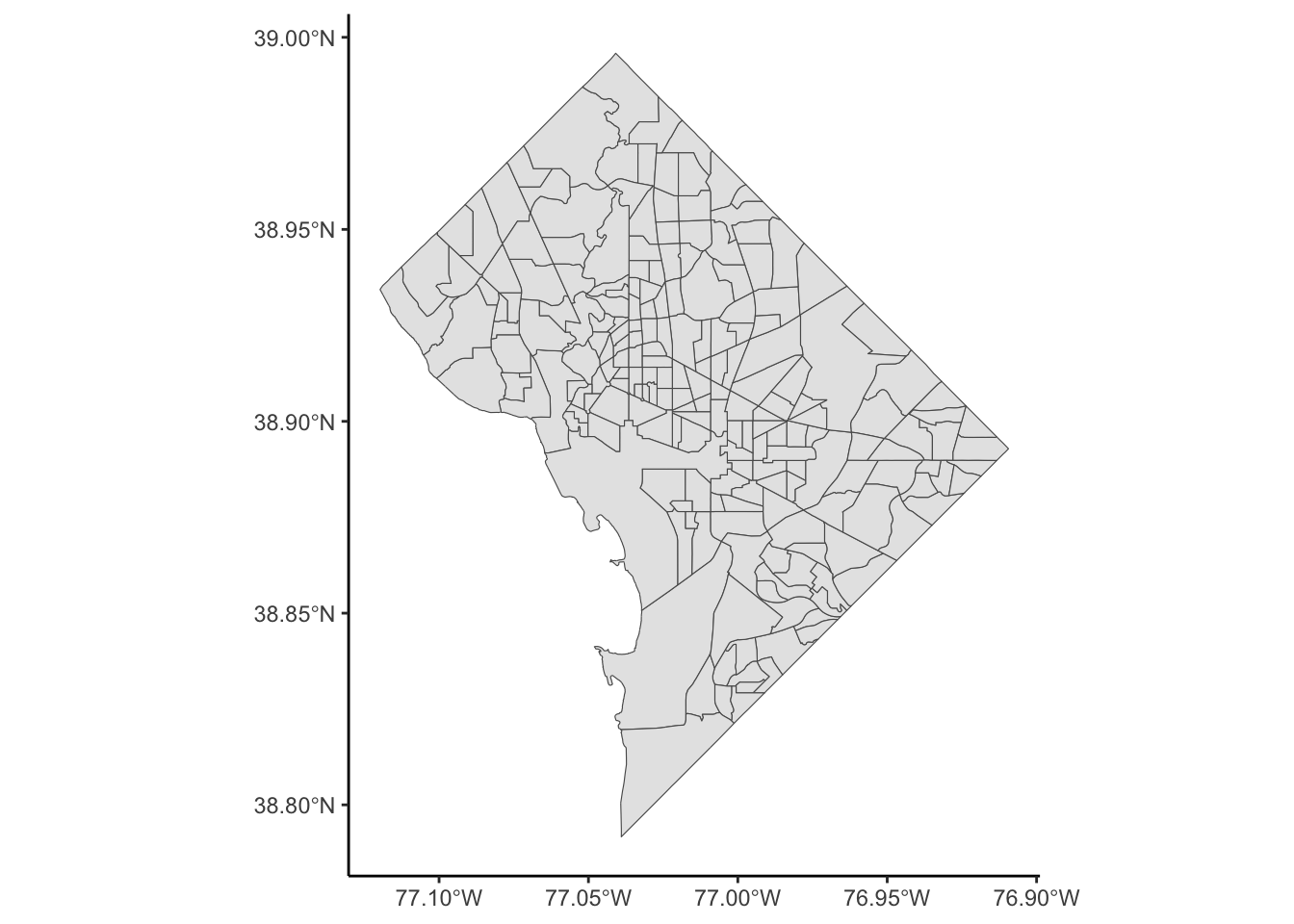

Vector \(\rightarrow\) Raster Data

Raster Data

• Each DC Census Tract has its own (odd) shape, which can be described by discrete coordinates forming a POLYGON
• For geospatial analysis, however, we often need to compute over evenly-spaced grids rather than this odd collection of shapes
  • Most common example: photos taken from an airplane/satellite! [Remote sensing]
• POLYGONs may make sense for demographers, but how about someone studying air pollution in DC? (Smog, for example, does not confine itself to census tracts!)

Step 1: Union of All Tracts

dc_union_sf <- sf::st_union(dc_sf)
dc_union_sf |>
  ggplot() +
  geom_sf() +
  theme_classic()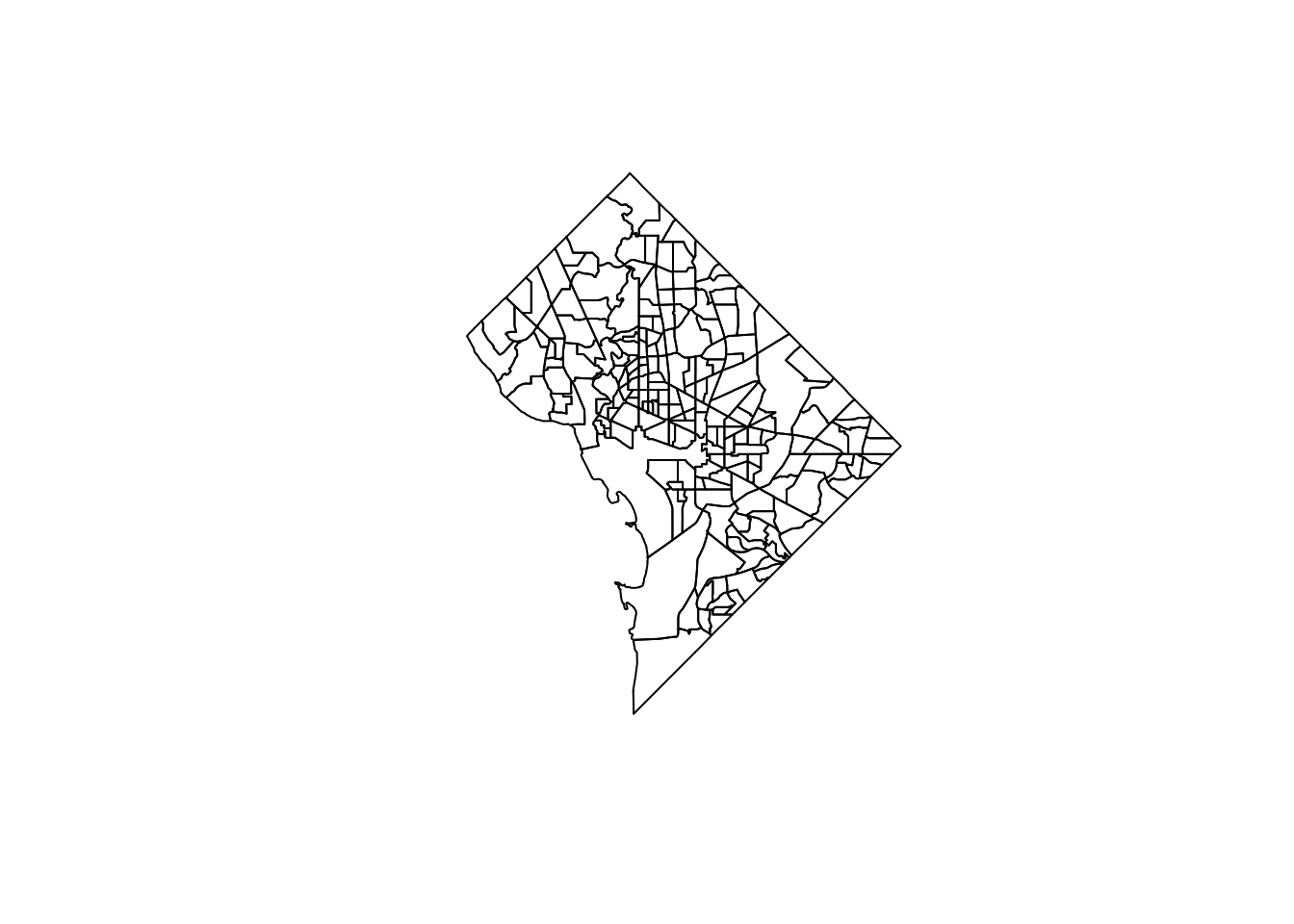

Step 2: Rasterize (terra)

library(terra)

terra 1.7.78

Attaching package: 'terra'

The following object is masked from 'package:tidyr':

    extract

dc_SpatVector <- terra::vect(dc_union_sf)
rast_template <- rast(ext(dc_SpatVector), resolution = 1000, crs = crs(dc_SpatVector))
dc_SpatRaster <- terra::rasterize(dc_SpatVector, rast_template)
dim(dc_SpatRaster)

[1] 29 23  1

plot(dc_SpatRaster)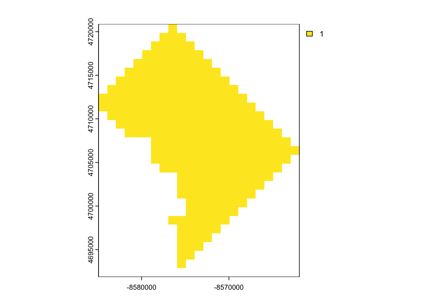

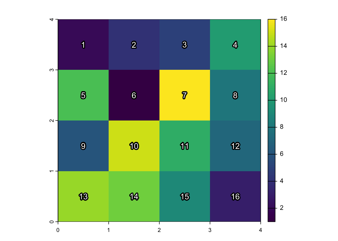
Rasters From Scratch

Welcome to Gridtown!

set.seed(6805)
library(terra)
gridtown <- terra::rast(
  nrows = 4, ncols = 4,
  xmin = 0, xmax = 4, ymin = 0, ymax = 4,
  vals = sample(1:16)
)
plot(gridtown)
text(
  gridtown,
  labels=1:16,
  halo=TRUE, hc="black", col="white", hw=0.2
)

Figure 3: Gridtown Indices

• Raster indices vs. values: The above plot displays indices for each cell: since a raster is a regular grid, can achieve memory-efficient representation with a single index (rather than, e.g., \((x, y)\) coords). But what we really care about are…

Raster Layer Values

plot(gridtown)
text(gridtown, halo=TRUE, hc="black", col="white", hw=0.2)

Figure 4: Gridtown Values

First Things First: Coordinates

• We need a way to unambiguously specify where things are on the earth

Latitude and Longitude are Angles!

From Krygier and Wood (2016)

Angular Distance vs. Travel Distance

The Earth’s “width” is slightly greater than its “length” 😰

From Wikimedia Commons

Projections

Smooshing 3D into 2D

From Monmonier (2018)

Avoid Getting Lost in the Sauce

How To Avoid Getting Lost in the Sauce

Tissot Circles: Imagine infinitely small ellipses placed at regular intervals on the curved surface of the earth. Imagine these ellipses being projected along with the earth’s surface. When scaled up, changes in the ellipses show the location and quality of distortions on the projected map.

The Things We Put On Maps

• Scales
• Points
• Lines
• Areas

Scales (w/Rules of Thumb)

From Krygier and Wood (2016)

The Three Key Elements

From Monmonier (2018)

Thought Experiment: Zooming In and Out

• What happens to points, lines, and areas?

What Can Happen to Points?

From Monmonier (2018)

What Can Happen to Lines?

From Monmonier (2018)

What Can Happen to Lines?

Selection

In any map, most features from the human or natural environment are eliminated! (Krygier and Wood 2016)

Simplification

Within the features that do remain, eliminate details that are unnecessary with respect to audience/context (Krygier and Wood 2016)

What Can Happen to Areas?

From Monmonier (2018)

Areal Dimension Change

From Krygier and Wood (2016)

What Is Gained?

From Monmonier (2018)

What Is Lost?

From Monmonier (2018)

Who Is Affected?

From Monmonier (2018)

Choropleths for Good and Evil

Having Domain Knowledge of a Region

From XKCD

Crime in Mongolia

From Reddit

Population of Mongolia

From Wikimedia Commons

Exhibit A

From Monmonier (2018)

Exhibit B

From Monmonier (2018)

Finding GIS Data

• Draws heavily on Chapter 6: “R packages to download open spatial data”, in Moraga (2018), Spatial Statistics for Data Science: Theory and Practice with R

Country Boundaries

Key package: rnaturalearth

library(rnaturalearth)
library(sf)
library(ggplot2)
library(viridis)

Loading required package: viridisLite

library(patchwork)

Attaching package: 'patchwork'

The following object is masked from 'package:terra':

    area

map1 <- ne_countries(type = "countries", country = "Germany", scale = "medium", returnclass = "sf")
map2 <- rnaturalearth::ne_states("Germany", returnclass = "sf")
(ggplot(map1) + geom_sf()) + (ggplot(map2) + geom_sf())

Climate Data

Key package: geodata

library(geodata)
d <- worldclim_country(country = "Jamaica", var = "tmin",
                       path = tempdir())
terra::plot(mean(d), plg = list(title = "Min. temperature (C)"))

Elevation

Key packages: rnaturalearth + elevatr

library(rnaturalearth)
library(elevatr)

elevatr v0.99.0 NOTE: Version 0.99.0 of 'elevatr' uses 'sf' and 'terra'.  Use 
of the 'sp', 'raster', and underlying 'rgdal' packages by 'elevatr' is being 
deprecated; however, get_elev_raster continues to return a RasterLayer.  This 
will be dropped in future versions, so please plan accordingly.

library(terra)
map <- ne_countries(type = "countries", country = "Switzerland",
                    scale = "medium", returnclass = "sf")
d <- get_elev_raster(locations = map, z = 9, clip = "locations")

Mosaicing & Projecting

Clipping DEM to locations

Note: Elevation units are in meters.

terra::plot(rast(d), plg = list(title = "Elevation (m)"))

Street Maps

library(osmdata)

Data (c) OpenStreetMap contributors, ODbL 1.0. https://www.openstreetmap.org/copyright

placebb <- getbb("Barcelona")
hospitals <- placebb %>% opq() %>%
  add_osm_feature(key = "amenity", value = "hospital") %>%
  osmdata_sf()
motorways <- placebb %>% opq() %>%
  add_osm_feature(key = "highway", value = "motorway") %>%
  osmdata_sf()
library(leaflet)
leaflet() |>  addTiles() |>
  addPolylines(data = motorways$osm_lines, color = "black") |>
  addPolygons(data = hospitals$osm_polygons,
              label = hospitals$osm_polygons$name)

World Bank Dataverse

Key package: wbstats

library(wbstats)
d <- wb_data(indicator = "MO.INDEX.HDEV.XQ",
             start_date = 2011, end_date = 2011)
library(rnaturalearth)
library(mapview)
map <- ne_countries(continent = "Africa", returnclass = "sf")
map <- dplyr::left_join(map, d, by = c("iso_a3" = "iso3c"))
mapview(map, zcol = "MO.INDEX.HDEV.XQ")

References

Krygier, John, and Denis Wood. 2016. Making Maps, Third Edition: A Visual Guide to Map Design for GIS. Guilford Publications.

Monmonier, Mark. 2018. How to Lie with Maps. University of Chicago Press. https://www.dropbox.com/scl/fi/7rsqbxgge6llggnaf5tit/How-to-Lie-with-Maps-Third-Edition.pdf?rlkey=6rqxta7cjyq3oqdnskj4dtwj8&dl=1.

Montessori, Maria. 1916. Spontaneous Activity in Education: A Basic Guide to the Montessori Methods of Learning in the Classroom. Lulu Press.