Week 4: Unary and Binary Operations

PPOL 6805 / DSAN 6750: GIS for Spatial Data Science
Fall 2025

Class Sessions

Author

Affiliation

Jeff Jacobs

jj1088@georgetown.edu

Published

Tuesday, September 17, 2024

Open slides in new tab →

Quick Logistical Things

HW1 Question 1 Clarifications
“Public Tests” vs. Hidden Tests

HW1 Question 1 Generally

“Simplest” / Most Efficient Representation

“Indicate which of the seven geometries above would provide the simplest representation of the entity”
GEOMETRYCOLLECTION could represent any of the geographic entities in Q1, but would be overkill for representing e.g. a single point or line

HW1 Question 1.8 Specifically

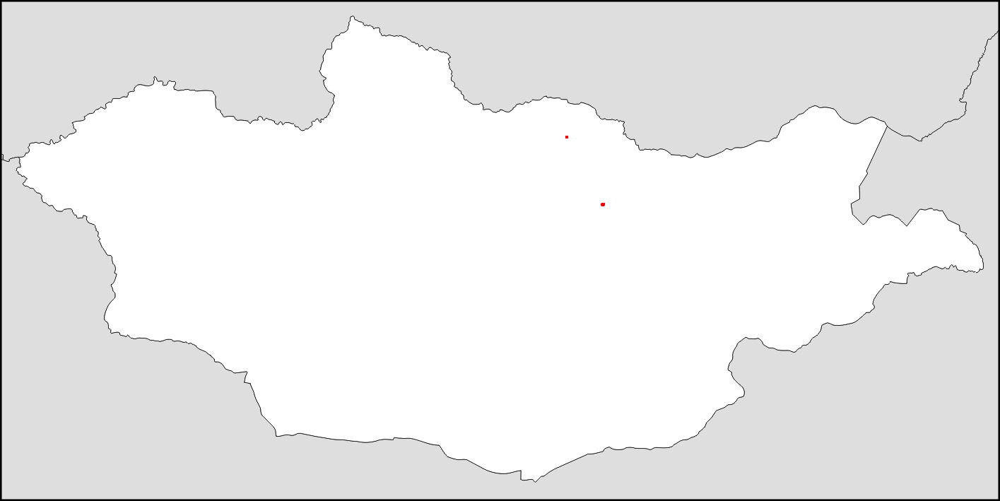
For the United Arab Emirates (UAE) data… we have what we call the Not-Paraguay-Problem: Most countries, including the UAE, have a bunch of lil “pieces”:

Code

ru_national_map <- ne_countries(type = "countries", country = "Russia", scale = "medium", returnclass = "sf")
mapview(ru_national_map)

Code

uae_national_map <- ne_countries(type = "countries", country = "United Arab Emirates", scale = "large", returnclass = "sf")
mapview(uae_national_map)

So, for Q1.8: Assume we’re just trying to have the computer represent the “mainland” (the biggest contiguous landmass, with Dubai on it!)

Public vs. Hidden Tests

Public Tests are basically “Quality Assurance Test”
Hidden Tests check for correctness

Coordinate Reference Systems

First things first… what are coordinates?
We need a way to unambiguously specify where things are on the earth

Latitude and Longitude are Angles!

From Krygier and Wood (2016)

Angular Distance vs. Travel Distance

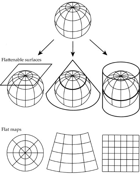
The Earth’s “width” is slightly greater than its “length” 😰

From Wikimedia Commons

Projections

Smooshing 3D into 2D

From Monmonier (2018)

Avoid Getting Lost in the Sauce

How To Avoid Getting Lost in the Sauce

Tissot Circles: Imagine infinitely small ellipses placed at regular intervals on the curved surface of the earth. Imagine these ellipses being projected along with the earth’s surface. When scaled up, changes in the ellipses show the location and quality of distortions on the projected map.

Choropleths for Good and Evil

Crucial crucial aspect of GIS: Having Domain Knowledge of a Region

The US’s Ur-Choropleth #1: Population

Kieran Healy, “America’s Ur-Choropleths”

The US’s Ur-Choropleth #2: Race

Kieran Healy, “America’s Ur-Choropleths”

Crime in Mongolia

From Reddit

Population of Mongolia

From Wikimedia Commons

Exhibit A

From Monmonier (2018)

Exhibit B

From Monmonier (2018)

Continuous Choropleth

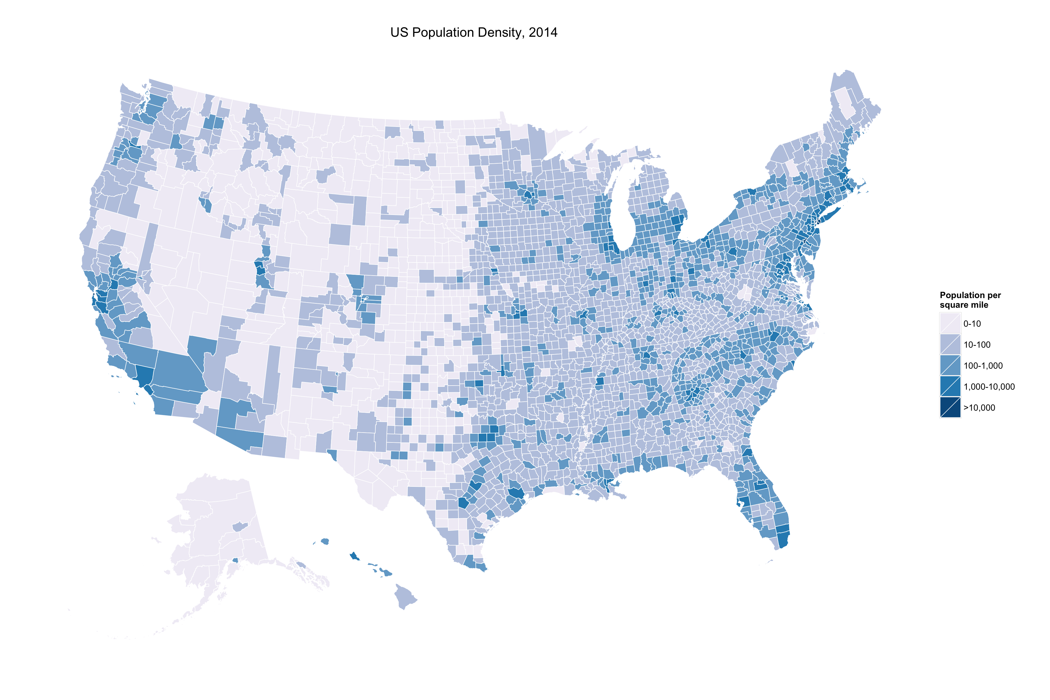
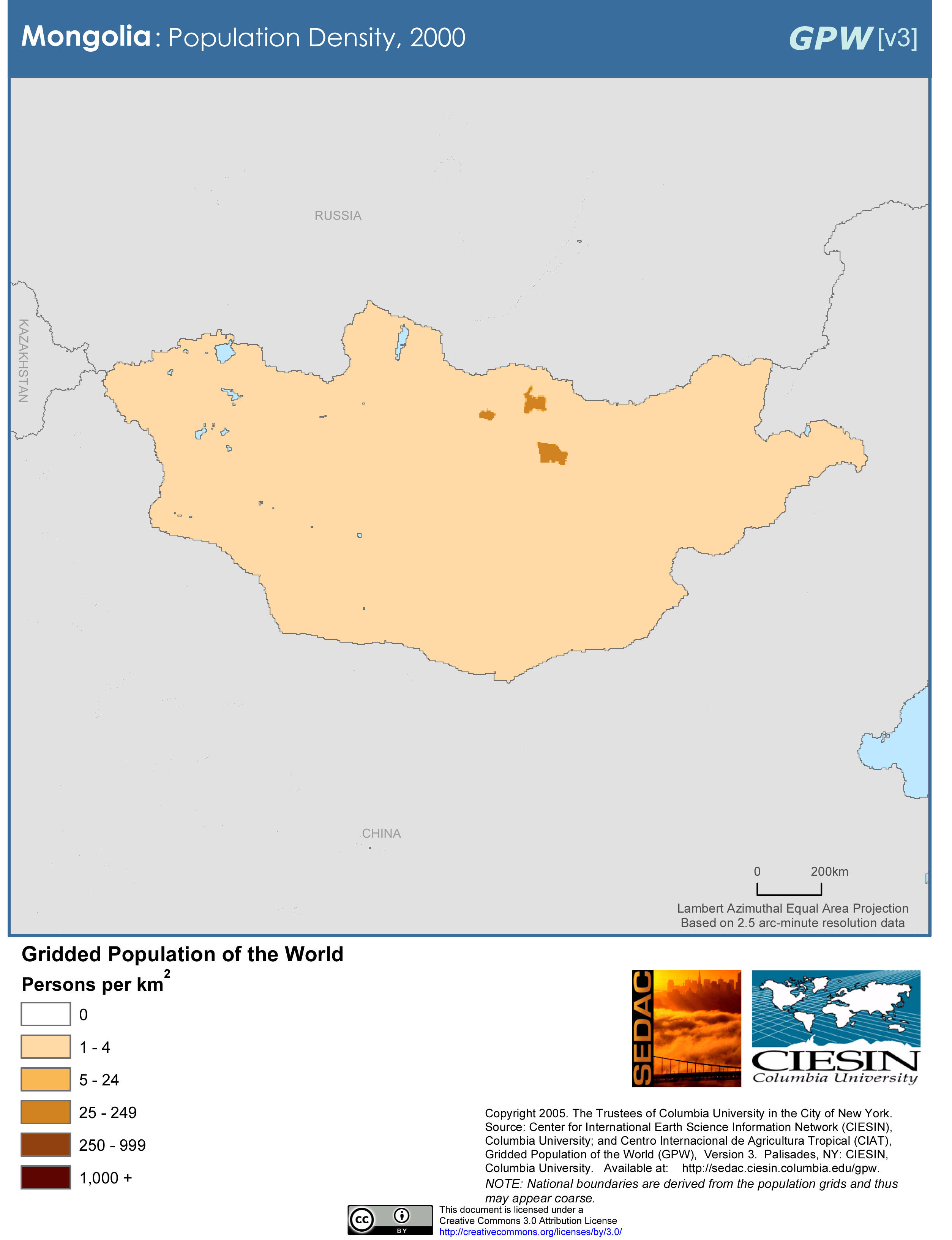
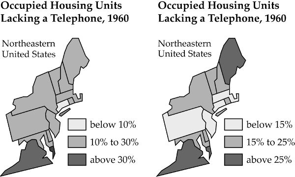
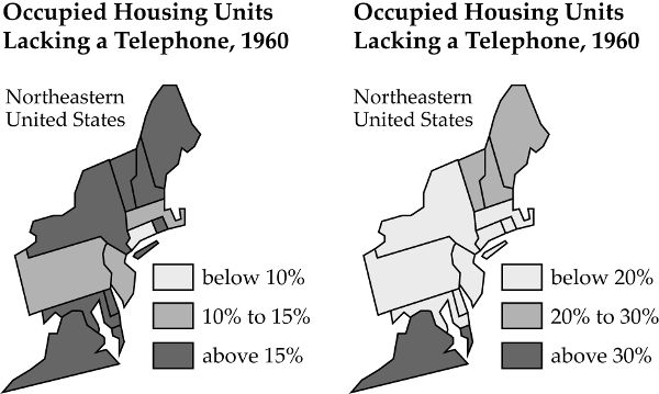
Is poverty a “significant issue” in the US?

From Krygier and Wood (2016)

Quantile Colormap

Is poverty a “significant issue” in the US?

Assigns the same number of observations to each color

From Krygier and Wood (2016)

Equal-Area Colormap

Is poverty a “significant issue” in the US?

Boundaries between colors come at regular (equal) intervals

From Krygier and Wood (2016)

Natural-Break Colormap

Is poverty a “significant issue” in the US?

Clustering algorithm chooses classes to (a) minimize differences within classes, (b) maximize differences between classes

From Krygier and Wood (2016)

Context-Sensitive Colormap

Is poverty a “significant issue” in the US?

A government program offers special funding for counties with above 25% poverty

From Krygier and Wood (2016)

The Importance of History

Is poverty a “significant issue” in the US?

From Krygier and Wood (2016)

Geospatial Operations 1: Unary Operations

Getting the Geometries

Using rnaturalearth with mapview

Code

set.seed(6805)
library(tidyverse)

── Attaching core tidyverse packages ──────────────────────── tidyverse 2.0.0 ──
✔ dplyr     1.1.4     ✔ readr     2.1.5
✔ forcats   1.0.0     ✔ stringr   1.5.1
✔ lubridate 1.9.4     ✔ tibble    3.3.0
✔ purrr     1.0.4     ✔ tidyr     1.3.1
── Conflicts ────────────────────────────────────────── tidyverse_conflicts() ──
✖ dplyr::filter() masks stats::filter()
✖ dplyr::lag()    masks stats::lag()
ℹ Use the conflicted package (<http://conflicted.r-lib.org/>) to force all conflicts to become errors

Code

library(sf)

Linking to GEOS 3.11.0, GDAL 3.5.3, PROJ 9.1.0; sf_use_s2() is TRUE

Code

library(rnaturalearth)
library(mapview)
france_sf <- ne_countries(country = "France", scale = 50)
(france_map <- mapview(france_sf, label = "geounit", legend = FALSE))

Centroid of France

Code

france_cent_sf <- sf::st_centroid(france_sf)

Warning: st_centroid assumes attributes are constant over geometries

Code

france_map + mapview(france_cent_sf, label = "Centroid", legend = FALSE)

One We Already Saw: Union

Computing the union of all geometries in the sf via sf::st_union()

Code

library(leaflet.extras2)

Loading required package: leaflet

Code

africa_sf <- ne_countries(continent = "Africa", scale = 50)
africa_union_sf <- sf::st_union(africa_sf)
africa_map <- mapview(africa_sf, label="geounit", legend=FALSE)
africa_union_map <- mapview(africa_union_sf, label="st_union(africa)", legend=FALSE)
africa_map | africa_union_map

Helpful for Rasterizing: BBox

Code

africa_bbox_sf <- sf::st_bbox(africa_sf)
africa_bbox_map <- mapview(africa_bbox_sf, label="st_bbox(africa)", legend=FALSE)
africa_map | africa_bbox_map

Convex Hulls by Country

Code

africa_countries_cvx <- sf::st_convex_hull(africa_sf)
africa_countries_cvx_map <- mapview(africa_countries_cvx, label="geounit", legend=FALSE)
africa_map | africa_countries_cvx_map

Convex Hull of Continent

Use st_union() first:

Code

africa_cvx <- africa_sf |> st_union() |> st_convex_hull()
africa_cvx_map <- mapview(africa_cvx, label="geounit", legend=FALSE)
africa_map | africa_cvx_map

One We Already Saw: Centroids

Computing the centroid of all geometries in the sf via sf::st_centroid()

Code

africa_cents_sf <- sf::st_centroid(africa_sf)

Warning: st_centroid assumes attributes are constant over geometries

Code

africa_cents_map <- mapview(africa_cents_sf, label="geounit", legend=FALSE)
africa_map | africa_cents_map

References

Krygier, John, and Denis Wood. 2016. Making Maps, Third Edition: A Visual Guide to Map Design for GIS. Guilford Publications.

Monmonier, Mark. 2018. How to Lie with Maps. University of Chicago Press. https://www.dropbox.com/scl/fi/7rsqbxgge6llggnaf5tit/How-to-Lie-with-Maps-Third-Edition.pdf?rlkey=6rqxta7cjyq3oqdnskj4dtwj8&dl=1.