Week 5: Binary Operations and DE-9IM

PPOL 6805 / DSAN 6750: GIS for Spatial Data Science
Fall 2025

Class Sessions
Author
Affiliation

Jeff Jacobs

Published

Wednesday, September 25, 2024

Open slides in new tab →

Geospatial Operations 2: Binary Operations

Spatial Joins

Code
africa_sf <- ne_countries(continent = "Africa", scale = 50)
africa_union_sf <- sf::st_union(africa_sf)
africa_map <- mapview(africa_sf, label="geounit", legend=FALSE)
nc <- system.file("shape/nc.shp", package="sf") |>
  read_sf() |>
  st_transform('EPSG:2264')
gr <- st_sf(
         label = apply(expand.grid(1:10, LETTERS[10:1])[,2:1], 1, paste0, collapse = ""),
         geom = st_make_grid(nc))
gr$col <- sf.colors(10, categorical = TRUE, alpha = .3)
# cut, to verify that NA's work out:
gr <- gr[-(1:30),]
suppressWarnings(nc_j <- st_join(nc, gr, largest = TRUE))
par(mfrow = c(2,1), mar = rep(0,4))
plot(st_geometry(nc_j), border = 'grey')
plot(st_geometry(gr), add = TRUE, col = gr$col)
text(st_coordinates(st_centroid(st_geometry(gr))), labels = gr$label, cex = .85)
# the joined dataset:
plot(st_geometry(nc_j), border = 'grey', col = nc_j$col)
text(st_coordinates(st_centroid(st_geometry(nc_j))), labels = nc_j$label, cex = .7)
plot(st_geometry(gr), border = '#88ff88aa', add = TRUE)

Spatial Sampling

Code
# Sample random points
africa_points_list <- sf::st_sample(africa_union_sf, 10)
africa_points_sf <- sf::st_sf(africa_points_list)
africa_points_map <- mapview(africa_points_sf, label="Random Point", col.regions=cb_palette[1], legend=FALSE)
Warning in cbind(`Feature ID` = fid, mat): number of rows of result is not a
multiple of vector length (arg 1)
Code
africa_map + africa_points_map

The “Default” Predicate: st_intersects

Code
countries_w_points <- africa_sf[africa_points_sf,]
mapview(countries_w_points, label="geounit", legend=FALSE) + africa_points_map

Counting with lengths()

Code
country_inter <- sf::st_intersects(africa_sf, africa_points_sf)
# Computes point counts for each polygon
(num_intersections <- lengths(country_inter))
 [1] 0 1 0 0 0 0 0 3 0 1 0 0 0 0 0 0 0 0 0 1 0 0 0 0 1 0 1 0 0 0 0 0 0 0 0 0 0 0
[39] 0 0 0 0 0 0 1 0 0 0 0 0 0 0 1 0
Code
africa_sf <- africa_sf |> mutate(
  num_points = num_intersections
) |> arrange(geounit)
africa_sf |> select(geounit, num_points) |> head()
geounit num_points geometry
Algeria 0 MULTIPOLYGON (((8.576563 36…
Angola 1 MULTIPOLYGON (((13.07275 -4…
Benin 0 MULTIPOLYGON (((1.622656 6….
Botswana 0 MULTIPOLYGON (((25.25879 -1…
Burkina Faso 0 MULTIPOLYGON (((0.9004883 1…
Burundi 0 MULTIPOLYGON (((30.55361 -2…

Plotting with mapview

Code
mapview(africa_sf, zcol="num_points")

Plotting with ggplot2

Since we’re starting to get into data attributes rather than geometric features, switching to ggplot2 is recommended!

Code
africa_sf |> ggplot(aes(fill=num_points)) +
  geom_sf() +
  theme_classic()

One More Unary Operation: st_buffer()

  • Think about how you might answer questions like:
    • “How far is your house (POINT) from Manhattan (POLYGON)?”
    • “Are there any chemical plants within a mile of this building (POLYGON) / stretch of road (LINESTRING)?”
  • Lazy mode (my favorite mode): Compute distances from the centroid
  • GIS master mode: Construct the buffer!

On POLYGONs

Key line: manhattan_buffer_sf <- manhattan_union_sf |> st_buffer(dist = 1609.34) (1 mile \(\approx\) 1609.34 meters)

Code
library(tidyverse)
library(sf)
library(tidycensus)
library(tigris)
library(mapview)
options(tigris_use_cache = TRUE)
manhattan_sf <- get_acs(
  geography = "tract",
  variables = "B19013_001",
  state = "NY",
  county = "New York",
  year = 2020,
  geometry = TRUE,
  cb = FALSE
)
# Erase the island tracts real quick
island_tracts <- c(
  "Census Tract 1, New York County, New York",
  "Census Tract 2.02, New York County, New York"
)
manhattan_sf <- manhattan_sf |> filter(
  !(NAME %in% island_tracts)
)
# Union of all census tracts within the county
manhattan_union_sf <- st_union(manhattan_sf)
manhattan_union_map <- mapview(manhattan_union_sf, label="New York County")
# Construct buffer (1 mile ~= 1609.34 meters)
manhattan_buffer_sf <- manhattan_union_sf |> st_buffer(dist = 1609.34)
manhattan_buffer_map <- mapview(manhattan_buffer_sf, label="Buffer (1 Mile)", col.regions = cbPalette[1], legend = TRUE)
manhattan_buffer_map + manhattan_union_map

On LINESTRINGs

Code
library(tidyverse)
library(sf)
## st_buffer, style options (taken from rgeos gBuffer)
l1 = st_as_sfc("LINESTRING(0 0,1 5,4 5,5 2,8 2,9 4,4 6.5)")
op = par(mfrow=c(2,3))
plot(st_buffer(l1, dist = 1, endCapStyle="ROUND"), reset = FALSE, main = "endCapStyle: ROUND")
plot(l1,col='blue',add=TRUE)
plot(st_buffer(l1, dist = 1, endCapStyle="FLAT"), reset = FALSE, main = "endCapStyle: FLAT")
plot(l1,col='blue',add=TRUE)
plot(st_buffer(l1, dist = 1, endCapStyle="SQUARE"), reset = FALSE, main = "endCapStyle: SQUARE")
plot(l1,col='blue',add=TRUE)
plot(st_buffer(l1, dist = 1, nQuadSegs=1), reset = FALSE, main = "nQuadSegs: 1")
plot(l1,col='blue',add=TRUE)
plot(st_buffer(l1, dist = 1, nQuadSegs=2), reset = FALSE, main = "nQuadSegs: 2")
plot(l1,col='blue',add=TRUE)
plot(st_buffer(l1, dist = 1, nQuadSegs= 5), reset = FALSE, main = "nQuadSegs: 5")
plot(l1,col='blue',add=TRUE)

From the sf Documentation

What Makes Binary Operations “Fancier”?

Unary
  • st_centroid()
    • POLYGON \(\mapsto\) POINT
    • MULTIPOLYGON \(\mapsto\) POINT
  • st_convex_hull()
    • POLYGON \(\mapsto\) POLYGON
    • MULTIPOINT \(\mapsto\) POLYGON
Binary
  • st_intersection()
    • (POINT, POINT) \(\mapsto\) POINT | POINT EMPTY
    • (POLYGON, POLYGON) \(\mapsto\) POLYGON | LINESTRING | POINT | POLYGON EMPTY
  • st_is_empty() and st_dimension() become your new best friends 😉
  • st_is_empty(): Distinguishes between, e.g., POINT EMPTY and POINT(0 0)
  • st_dimension(): NA for empty versions, otherwise
    • 2 for surfaces (POLYGON, MULTIPOLYGON)
    • 1 for lines (LINESTRING, MULTILINESTRING)
    • 0 for points (POINT, MULTIPOINT)

The Bad Kind of Overthinking: Will My Life Just Get Harder and Harder?

Unary Operations

Binary Operations

Ternary Operations

Quaternary Operations

Good News and Bad News

  • The good news: No!
  • The bad news: You’ll have to read the 465-page Volume I and then the 451-page Volume II and then to page 15 of Volume III of Cohn (1965) to know why:

(i spent 4 yrs of undergrad studying abstract algebra and now it all sits gathering dust somewhere deep within my brain plz just let me have this moment i’ll never mention it again i promise)

The Good Kind of Overthinking…

  • For fancier geospatial operations, we’ll need to start overthinking, about the possible relationships between two (or more) geometries! \(\leadsto\) Relational Predicates:

Figure 4.2 in Lovelace, Nowosad, and Muenchow (2024)

Ad Hoc / Ambiguous \(\rightarrow\) Precise: Enter DE-9IM!

DE-9IM Strings

Each cell here visualizes one component of the DE-9IM string 1020F1102, which describes the relationship between the following two geometries:

  • Boxey McBoxface: POLYGON(0 0, 1 0, 1 1, 0 1, 0 0)
  • Liney McLineface: LINESTRING(0.5 -0.5, 0.5 0.5)
Code
library(sf)
polygon <- po <- st_polygon(list(rbind(c(0,0), c(1,0), c(1,1), c(0,1), c(0,0))))
p0 <- st_polygon(list(rbind(c(-1,-1), c(2,-1), c(2,2), c(-1,2), c(-1,-1))))
line <- li <- st_linestring(rbind(c(.5, -.5), c(.5, 0.5)))
s <- st_sfc(po, li)

par(mfrow = c(3,3))
par(mar = c(1,1,1,1))
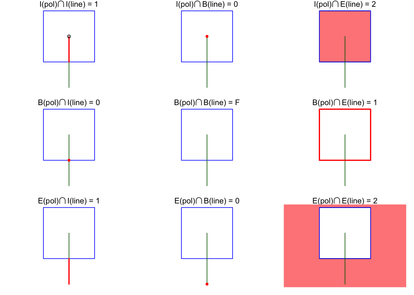
# "1020F1102"
# 1: 1
plot(s, col = c(NA, 'darkgreen'), border = 'blue', main = expression(paste("I(pol)",intersect(),"I(line) = 1")))
lines(rbind(c(.5,0), c(.5,.495)), col = 'red', lwd = 2)
points(0.5, 0.5, pch = 1)

# 2: 0
plot(s, col = c(NA, 'darkgreen'), border = 'blue', main = expression(paste("I(pol)",intersect(),"B(line) = 0")))
points(0.5, 0.5, col = 'red', pch = 16)

# 3: 2
plot(s, col = c(NA, 'darkgreen'), border = 'blue', main = expression(paste("I(pol)",intersect(),"E(line) = 2")))
plot(po, col = '#ff8888', add = TRUE)
plot(s, col = c(NA, 'darkgreen'), border = 'blue', add = TRUE)

# 4: 0
plot(s, col = c(NA, 'darkgreen'), border = 'blue', main = expression(paste("B(pol)",intersect(),"I(line) = 0")))
points(.5, 0, col = 'red', pch = 16)

# 5: F
plot(s, col = c(NA, 'darkgreen'), border = 'blue', main = expression(paste("B(pol)",intersect(),"B(line) = F")))

# 6: 1
plot(s, col = c(NA, 'darkgreen'), border = 'blue', main = expression(paste("B(pol)",intersect(),"E(line) = 1")))
plot(po, border = 'red', col = NA, add = TRUE, lwd = 2)

# 7: 1
plot(s, col = c(NA, 'darkgreen'), border = 'blue', main = expression(paste("E(pol)",intersect(),"I(line) = 1")))
lines(rbind(c(.5, -.5), c(.5, 0)), col = 'red', lwd = 2)

# 8: 0
plot(s, col = c(NA, 'darkgreen'), border = 'blue', main = expression(paste("E(pol)",intersect(),"B(line) = 0")))
points(.5, -.5, col = 'red', pch = 16)

# 9: 2
plot(s, col = c(NA, 'darkgreen'), border = 'blue', main = expression(paste("E(pol)",intersect(),"E(line) = 2")))
plot(p0 / po, col = '#ff8888', add = TRUE)
plot(s, col = c(NA, 'darkgreen'), border = 'blue', add = TRUE)

Code from Pebesma and Bivand (2023)
  • The predicate equals corresponds to the DE-9IM string "T*F**FFF*". If any two geometries obey this relationship, they are (topologically) equal!

Slowing Down: 9IM (no DE yet!)

Table 1: From OSGeo Project
9IM Interior Boundary Exterior
Interior


Boundary


Exterior


Dimensionally Extended (DE) 9IM

Table 2: From OSGeo Project
9IM Interior Boundary Exterior
Interior
2

1

2
Boundary
1

0

1
Exterior
2

1

2

Crunching it Down into a Tiny Box

DE-9IM Interior Boundary Exterior
Interior 2 1 2
Boundary 1 0 1
Exterior 2 1 2

And Then into a Tiny String

212101212

And Then into an Infinitesimally-Small Point

DE-9IM Masks

  • Now terms can be given unambiguous, precise meaning!
st_overlaps() Interior Boundary Exterior
Interior T * T
Boundary * * *
Exterior T * *
  • Special Values (besides 0, 1, 2):
    • T: “True” (non-empty, st_dimension() >= 0)
    • F: “False” (empty, st_dimension() == NA)
    • *: “Wildcard” (Don’t care what the value is)
  • st_overlaps(): T*T***T**, st_equals(): T*F**FFF*

DE-9IM vs. Everyday Language

  • DE-9IM can (in theory) represent \(6^9 = 10~077~696\) possible geometric relationships!
  • The English language has like 10, and they’re ambiguous ☠️ (Compromise employed by GIS systems: allow multiple masks for same English word:)
English Mask 212101212 Result
“Disjoint” FF*FF**** FALSE x not disjoint from y
“Touches” FT******* FALSE x doesn’t touch y
“Touches” F***T**** FALSE x doesn’t touch y
“Crosses” T*T***T** TRUE x crosses y
“Within” TF*F***** FALSE x is not within y
“Overlaps” T*T***T** TRUE x overlaps y

st_relate(): The Ultimate Predicate

Code
library(tidyverse)
library(rnaturalearth)
us <- ne_states(country="United States of America")
dc <- us |> filter(iso_3166_2 == "US-DC")
us <- us |>
  mutate(
    de9im = st_relate(us, dc),
    touch = st_touches(us, dc, sparse = F)
  ) |>
  select(iso_3166_2, name, de9im, touch) |>
  arrange(name)
although coordinates are longitude/latitude, st_relate assumes that they are
planar
Code
us
iso_3166_2 name de9im touch geometry
US-AL Alabama FF2FF1212 FALSE MULTIPOLYGON (((-87.41958 3…
US-AK Alaska FF2FF1212 FALSE MULTIPOLYGON (((-141.0056 6…
US-AZ Arizona FF2FF1212 FALSE MULTIPOLYGON (((-111.0063 3…
US-AR Arkansas FF2FF1212 FALSE MULTIPOLYGON (((-90.30422 3…
US-CA California FF2FF1212 FALSE MULTIPOLYGON (((-114.7243 3…
US-CO Colorado FF2FF1212 FALSE MULTIPOLYGON (((-109.0463 4…
US-CT Connecticut FF2FF1212 FALSE MULTIPOLYGON (((-73.6417 41…
US-DE Delaware FF2FF1212 FALSE MULTIPOLYGON (((-75.05809 3…
US-DC District of Columbia 2FFF1FFF2 FALSE MULTIPOLYGON (((-77.02293 3…
US-FL Florida FF2FF1212 FALSE MULTIPOLYGON (((-87.44734 3…
US-GA Georgia FF2FF1212 FALSE MULTIPOLYGON (((-80.89029 3…
US-HI Hawaii FF2FF1212 FALSE MULTIPOLYGON (((-154.8996 1…
US-ID Idaho FF2FF1212 FALSE MULTIPOLYGON (((-117.0382 4…
US-IL Illinois FF2FF1212 FALSE MULTIPOLYGON (((-89.1237 36…
US-IN Indiana FF2FF1212 FALSE MULTIPOLYGON (((-84.80608 4…
US-IA Iowa FF2FF1212 FALSE MULTIPOLYGON (((-96.48266 4…
US-KS Kansas FF2FF1212 FALSE MULTIPOLYGON (((-102.0396 3…
US-KY Kentucky FF2FF1212 FALSE MULTIPOLYGON (((-89.42446 3…
US-LA Louisiana FF2FF1212 FALSE MULTIPOLYGON (((-89.52599 3…
US-ME Maine FF2FF1212 FALSE MULTIPOLYGON (((-71.08495 4…
US-MD Maryland FF2F11212 TRUE MULTIPOLYGON (((-75.64786 3…
US-MA Massachusetts FF2FF1212 FALSE MULTIPOLYGON (((-71.19396 4…
US-MI Michigan FF2FF1212 FALSE MULTIPOLYGON (((-84.4913 46…
US-MN Minnesota FF2FF1212 FALSE MULTIPOLYGON (((-97.22609 4…
US-MS Mississippi FF2FF1212 FALSE MULTIPOLYGON (((-88.40221 3…
US-MO Missouri FF2FF1212 FALSE MULTIPOLYGON (((-95.31725 4…
US-MT Montana FF2FF1212 FALSE MULTIPOLYGON (((-116.0482 4…
US-NE Nebraska FF2FF1212 FALSE MULTIPOLYGON (((-104.0537 4…
US-NV Nevada FF2FF1212 FALSE MULTIPOLYGON (((-114.0425 4…
US-NH New Hampshire FF2FF1212 FALSE MULTIPOLYGON (((-71.50585 4…
US-NJ New Jersey FF2FF1212 FALSE MULTIPOLYGON (((-75.54133 3…
US-NM New Mexico FF2FF1212 FALSE MULTIPOLYGON (((-108.1375 3…
US-NY New York FF2FF1212 FALSE MULTIPOLYGON (((-79.06523 4…
US-NC North Carolina FF2FF1212 FALSE MULTIPOLYGON (((-76.03173 3…
US-ND North Dakota FF2FF1212 FALSE MULTIPOLYGON (((-104.0476 4…
US-OH Ohio FF2FF1212 FALSE MULTIPOLYGON (((-80.52023 4…
US-OK Oklahoma FF2FF1212 FALSE MULTIPOLYGON (((-103.0002 3…
US-OR Oregon FF2FF1212 FALSE MULTIPOLYGON (((-124.4924 4…
US-PA Pennsylvania FF2FF1212 FALSE MULTIPOLYGON (((-79.76301 4…
US-RI Rhode Island FF2FF1212 FALSE MULTIPOLYGON (((-71.23686 4…
US-SC South Carolina FF2FF1212 FALSE MULTIPOLYGON (((-78.57316 3…
US-SD South Dakota FF2FF1212 FALSE MULTIPOLYGON (((-104.0567 4…
US-TN Tennessee FF2FF1212 FALSE MULTIPOLYGON (((-90.30422 3…
US-TX Texas FF2FF1212 FALSE MULTIPOLYGON (((-103.3115 2…
US-UT Utah FF2FF1212 FALSE MULTIPOLYGON (((-111.0502 4…
US-VT Vermont FF2FF1212 FALSE MULTIPOLYGON (((-73.35134 4…
US-VA Virginia FF2F11212 TRUE MULTIPOLYGON (((-76.01325 3…
US-WA Washington FF2FF1212 FALSE MULTIPOLYGON (((-122.753 48…
US-WV West Virginia FF2FF1212 FALSE MULTIPOLYGON (((-82.58945 3…
US-WI Wisconsin FF2FF1212 FALSE MULTIPOLYGON (((-87.80425 4…
US-WY Wyoming FF2FF1212 FALSE MULTIPOLYGON (((-109.0463 4…

(If You Don’t Want to Scroll)

Code
us |> filter(touch)
Warning: Using one column matrices in `filter()` was deprecated in dplyr 1.1.0.
ℹ Please use one dimensional logical vectors instead.
iso_3166_2 name de9im touch geometry
US-MD Maryland FF2F11212 TRUE MULTIPOLYGON (((-75.64786 3…
US-VA Virginia FF2F11212 TRUE MULTIPOLYGON (((-76.01325 3…

References

Cohn, P. M. 1965. Universal Algebra. Springer Science & Business Media.
Lovelace, Robin, Jakub Nowosad, and Jannes Muenchow. 2024. Geocomputation with R. CRC Press. https://r.geocompx.org/.
Pebesma, Edzer, and Roger Bivand. 2023. Spatial Data Science: With Applications in R. CRC Press. https://r-spatial.org/book/.