Code
user_df.head()| read_time | dark_mode | male | age | hours | |
|---|---|---|---|---|---|
| 0 | 14.4 | False | 0 | 43.0 | 65.6 |
| 1 | 15.4 | False | 1 | 55.0 | 125.4 |
| 2 | 20.9 | True | 0 | 23.0 | 642.6 |
| 3 | 20.0 | False | 0 | 41.0 | 129.1 |
| 4 | 21.5 | True | 0 | 29.0 | 190.2 |
DSAN 5650: Causal Inference for Computational Social Science
Summer 2026, Georgetown University
Today’s Planned Schedule:
| Start | End | Topic | |
|---|---|---|---|
| Lecture | 6:30pm | 6:45pm | Final Projects → |
| 6:45pm | 7:10pm | Instrumental Variables Lite → | |
| 7:30pm | 8:00pm | When Conditioning Won’t Cut It: IVs → | |
| 7:10pm | 8:00pm | Text-as-Data Part 1: TAD in General → | |
| Break! | 8:00pm | 8:10pm | |
| 8:10pm | 9:00pm | Text-as-Data Part 2: Causal Text Analysis → |
\[ \DeclareMathOperator*{\argmax}{argmax} \DeclareMathOperator*{\argmin}{argmin} \newcommand{\bigexp}[1]{\exp\mkern-4mu\left[ #1 \right]} \newcommand{\bigexpect}[1]{\mathbb{E}\mkern-4mu \left[ #1 \right]} \newcommand{\definedas}{\overset{\small\text{def}}{=}} \newcommand{\definedalign}{\overset{\phantom{\text{defn}}}{=}} \newcommand{\eqeventual}{\overset{\text{eventually}}{=}} \newcommand{\Err}{\text{Err}} \newcommand{\expect}[1]{\mathbb{E}[#1]} \newcommand{\expectsq}[1]{\mathbb{E}^2[#1]} \newcommand{\fw}[1]{\texttt{#1}} \newcommand{\given}{\mid} \newcommand{\green}[1]{\color{green}{#1}} \newcommand{\heads}{\outcome{heads}} \newcommand{\iid}{\overset{\text{\small{iid}}}{\sim}} \newcommand{\lik}{\mathcal{L}} \newcommand{\loglik}{\ell} \DeclareMathOperator*{\maximize}{maximize} \DeclareMathOperator*{\minimize}{minimize} \newcommand{\mle}{\textsf{ML}} \newcommand{\nimplies}{\;\not\!\!\!\!\implies} \newcommand{\orange}[1]{\color{orange}{#1}} \newcommand{\outcome}[1]{\textsf{#1}} \newcommand{\param}[1]{{\color{purple} #1}} \newcommand{\pgsamplespace}{\{\green{1},\green{2},\green{3},\purp{4},\purp{5},\purp{6}\}} \newcommand{\pedge}[2]{\require{enclose}\enclose{circle}{~{#1}~} \rightarrow \; \enclose{circle}{\kern.01em {#2}~\kern.01em}} \newcommand{\pnode}[1]{\require{enclose}\enclose{circle}{\kern.1em {#1} \kern.1em}} \newcommand{\ponode}[1]{\require{enclose}\enclose{box}[background=lightgray]{{#1}}} \newcommand{\pnodesp}[1]{\require{enclose}\enclose{circle}{~{#1}~}} \newcommand{\purp}[1]{\color{purple}{#1}} \newcommand{\sign}{\text{Sign}} \newcommand{\spacecap}{\; \cap \;} \newcommand{\spacewedge}{\; \wedge \;} \newcommand{\tails}{\outcome{tails}} \newcommand{\Var}[1]{\text{Var}[#1]} \newcommand{\bigVar}[1]{\text{Var}\mkern-4mu \left[ #1 \right]} \]
🥳 You’re doing great 🥳

…So, is this a causal effect? Does dark theme cause users to spend less time reading?
(…since I couldn’t figure out how to fit it on the last slide)
import matplotlib
matplotlib.rcParams['axes.grid'] = False
matplotlib.rcParams['savefig.transparent'] = True
sns.pairplot(
  data=user_df,
  height=1.5, aspect=1.75,
)
plt.show()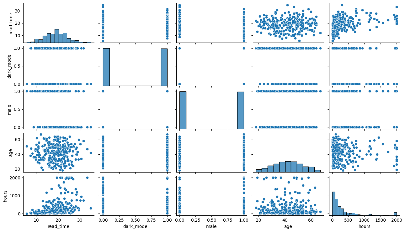
Enter Uber’s causal inference library: causalml
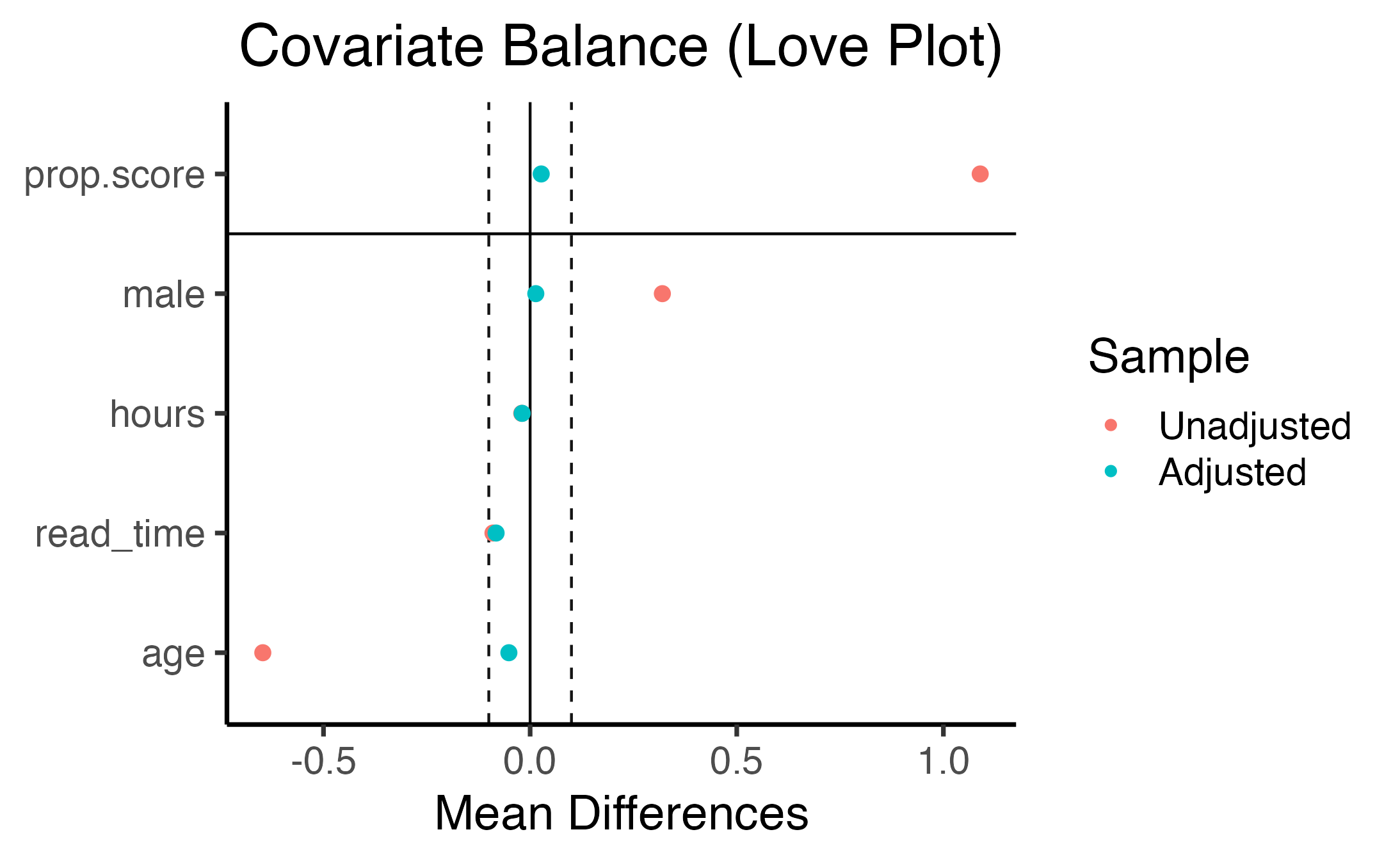
And then WeightIt to generate a “love plot”:
\[ \hat\tau = \frac{1}{n}\sum_i \left[ \hat\mu_1(X_i) - \hat\mu_0(X_i) + \frac{T_i(Y_i - \hat\mu_1(X_i))}{\hat e(X_i)} - \frac{(1-T_i)(Y_i - \hat\mu_0(X_i))}{1-\hat e(X_i)} \right] \]
def estimate_e(df, X, D, model_e):
    e = model_e.fit(df[X], df[D]).predict_proba(df[X])[:,1]
    return e
user_df['e'] = estimate_e(user_df, X, "dark_mode", LogisticRegression())
fig, ax = plt.subplots(figsize=(7,2.75))
sns.kdeplot(
  x='e', hue='dark_mode', data=user_df,
  # bins=30,
  #stat='density',
  common_norm=False,
  fill=True,
  ax=ax
);
ax.set_xlabel("$e(X)$");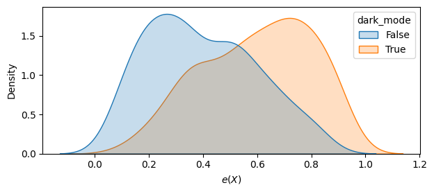
First, with scikit-learn:
Enter EconML, Microsoft’s “Official” ML-based econometrics library 😎
Wrong regression model:
def compare_estimators(X_e, X_mu, D, y, seed):
    df = generate_data(seed=seed)
    e = estimate_e(df, X_e, D, LogisticRegression())
    mu0, mu1 = estimate_mu(df, X_mu, D, y, LinearRegression())
    slearn = mu1 - mu0
    ipw = (df[D] / e - (1-df[D]) / (1-e)) * df[y]
    aipw = slearn + df[D] / e * (df[y] - mu1) - (1-df[D]) / (1-e) * (df[y] - mu0)
    return np.mean((slearn, ipw, aipw), axis=1)

def simulate_estimators(X_e, X_mu, D, y):
    r = Parallel(n_jobs=8)(delayed(compare_estimators)(X_e, X_mu, D, y, i) for i in range(100))
    df_tau = pd.DataFrame(r, columns=['S-learn', 'IPW', 'AIPW'])
    return df_tau
# The actual plots
fig, ax = plt.subplots(figsize=(4,3.5))
wrong_reg_df = simulate_estimators(
  X_e=['male', 'age'], X_mu=['hours'], D="dark_mode", y="read_time"
)
wrong_reg_plot = sns.boxplot(
  data=pd.melt(wrong_reg_df), x='variable', y='value', hue='variable',
  ax=ax,
  linewidth=2
);
wrong_reg_plot.set(
  title="Distribution of $\hat τ$", xlabel='', ylabel=''
);
ax.axhline(2, c='r', ls=':');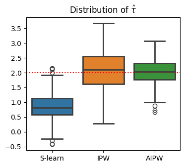
Wrong propensity score model:
fig, ax = plt.subplots(figsize=(4, 3.5))
wrong_ps_df = simulate_estimators(
  ['age'], ['male', 'hours'], D="dark_mode", y="read_time"
)
wrong_ps_plot = sns.boxplot(
  data=pd.melt(wrong_ps_df), x='variable', y='value', hue='variable',
  ax=ax,
  linewidth=2
);
ax.set_title("Distribution of $\hat τ$");
ax.axhline(2, c='r', ls=':');
plt.show()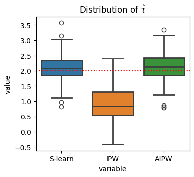
If randomization works to obtain causal effects…
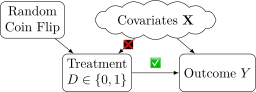
…Find something random in the causal system, use e.g. matching to “force” the same scenario!
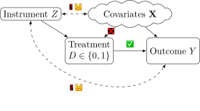
General form: \(\text{Effect}(D \rightarrow Y) = \frac{\text{Effect}(Z \rightarrow Y)}{\text{Effect}(Z \rightarrow D)}\) (Try “plugging in” \(Z\) = Coin Flip!)
\[ \beta_{\text{IV}}^{\text{Wald}} = \frac{ \mathbb{E}[Y_i \mid Z_i = 1] - \mathbb{E}[Y_i \mid Z_i = 0] }{ \mathbb{E}[D_i \mid Z_i = 1] - \mathbb{E}[D_i \mid Z_i = 0] }, \; \beta_{\text{IV}} = \frac{\text{Cov}[Y, Z]}{\text{Cov}[D,Z]} \]
(The necessity for sample splitting!)
| \(Y_i \mid \textsf{do}(D_i \leftarrow 1)\) | \(Y_i \mid \textsf{do}(D_i \leftarrow 0)\) | |
|---|---|---|
| Person 1 | Candidate’s Morals | Taxes |
| Person 2 | Candidate’s Morals | Taxes |
| Person 3 | Polarization | Immigration |
| Person 4 | Polarization | Immigration |
| \(Y_i \mid \textsf{do}(D_i \leftarrow 1)\) | \(Y_i \mid \textsf{do}(D_i \leftarrow 0)\) | |
|---|---|---|
| Person 1 | Candidate’s Morals | Taxes |
| Person 2 | Candidate’s Morals | Taxes |
| Person 3 | Polarization | Immigration |
| Person 4 | Polarization | Immigration |
| Actual Assignment | Outcome \(Y_i\) | |
|---|---|---|
| Person 1 | \(D_1 = 1\) | Morals |
| Person 2 | \(D_2 = 1\) | Morals |
| Person 3 | \(D_3 = 0\) | Immigration |
| Person 4 | \(D_4 = 0\) | Immigration |
| Actual Assignment | Outcome \(Y_i\) | |
|---|---|---|
| Person 1 | \(D_1 = 1\) | Morals |
| Person 2 | \(D_2 = 0\) | Taxes |
| Person 3 | \(D_3 = 1\) | Polarization |
| Person 4 | \(D_4 = 0\) | Immigration |
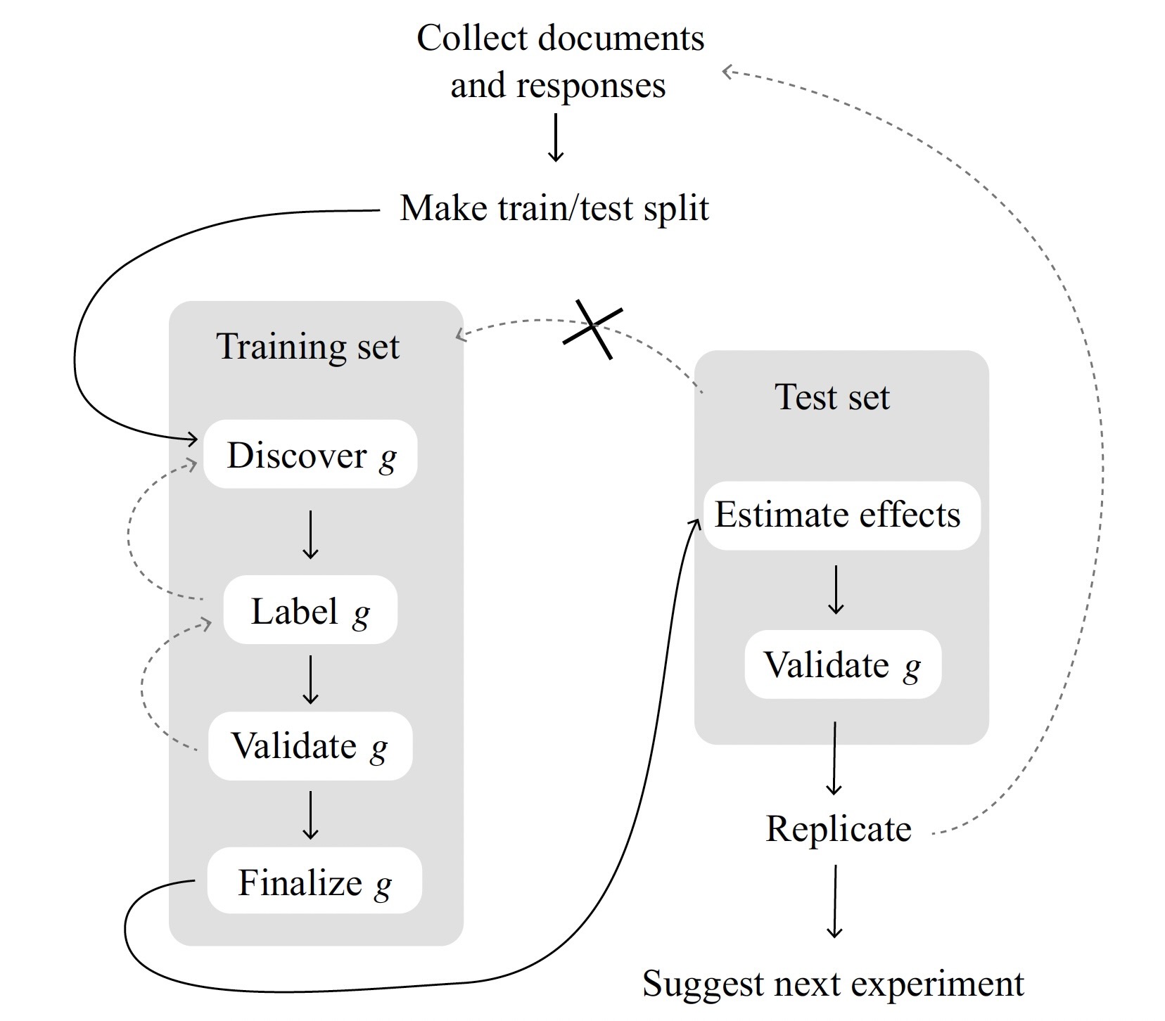
| Section | Keywords |
|---|---|
| U.S. News | state, court, federal, republican |
| World News | government, country, officials, minister |
| Arts | music, show, art, dance |
| Sports | game, league, team, coach |
| Real Estate | home, bedrooms, bathrooms, building |
| Arts | Real Estate | Sports | U.S. News | World News | |
|---|---|---|---|---|---|
| Correct | 3020 | 690 | 4860 | 1330 | 1730 |
| Incorrect | 750 | 60 | 370 | 1100 | 590 |
| Accuracy | 0.801 | 0.920 | 0.929 | 0.547 | 0.746 |
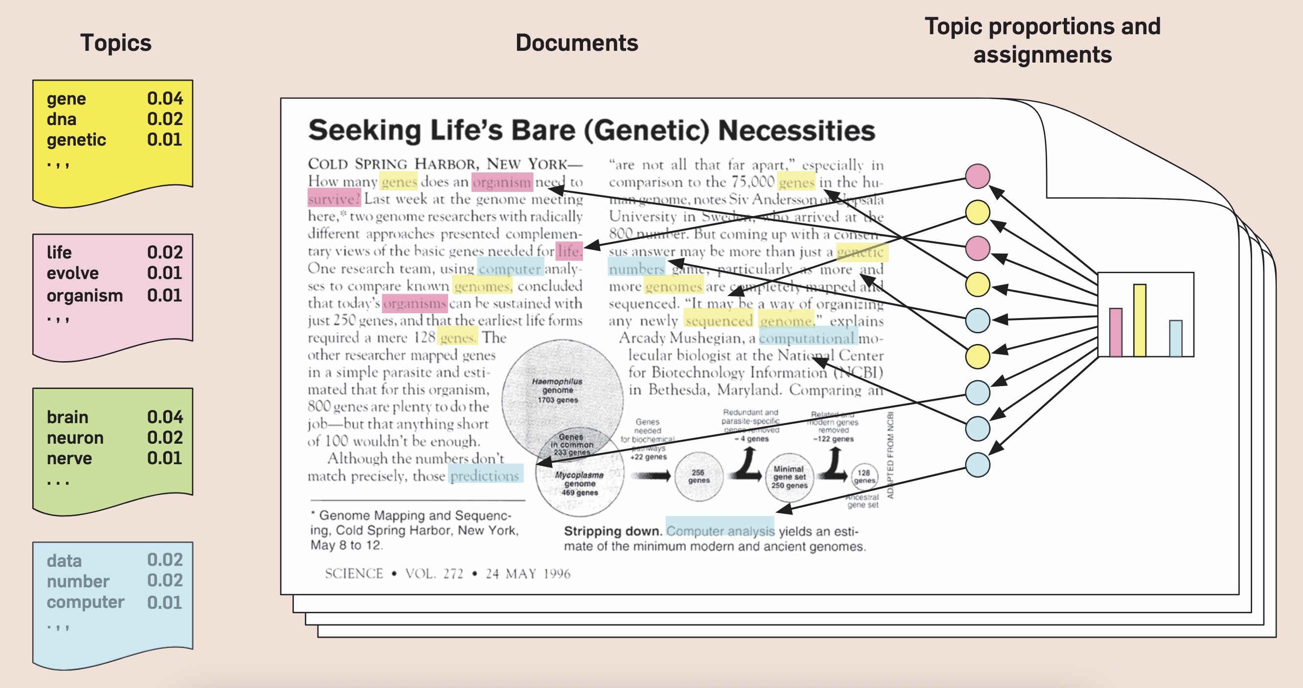
…Unlocks a world of social modeling through text!
Blaydes et al. (2018)