Syllabus
DSAN 5650: Causal Inference for Computational Social Science
Welcome to DSAN 5650: Causal Inference for Computational Social Science at Georgetown University!
The course meets on Wednesdays from 6:30-9pm online via Zoom
Course Staff
- Prof. Jeff Jacobs,
jj1088@georgetown.edu- Office hours (Click to schedule): Tuesdays, 3:30-6pm
- TA Noelle Martell,
nm1237@georgetown.edu- Office hours by appointment
Course Description
This course provides students with the opportunity to take the analytical skills, machine learning algorithms, and statistical methods learned throughout their first year in the program and explore how they can be employed to carry out rigorous, original research in the behavioral and social sciences. With a particular emphasis on tackling the additional challenges which arise when moving from associational to causal inference, particularly when only observational (as opposed to experimental) data is available, students will become proficient in cutting-edge causal Machine Learning techniques such as propensity score matching, synthetic controls, causal program evaluation, inverse social welfare function estimation from panel data, and Double-Debiased Machine Learning.
In-class examples will cover continuous, discrete-choice, and textual data from a wide swath of social and behavioral sciences: economics, political science, sociology, anthropology, quantitative history, and digital humanities. After gaining experience through in-class labs and homework assignments focused on reproducing key findings from recent journal articles in each of these disciplines, students will spend the final weeks of the course on a final project demonstrating their ability to develop, evaluate, and test the robustness of a causal hypothesis.
Prerequisites: DSAN 5000, DSAN 5100 (DSAN 5300 recommended but not required)
Course Overview
The fundamental building block for the course is the idea of a Data-Generating Process (DGP). You may have encountered this concept in passing during other DSAN courses (for example, in DSAN 5100, a phrase like “Assume \(X\) is drawn i.i.d. from a Normal distribution with mean \(\mu\) and variance \(\sigma^2\)” is a statement characterizing the DGP of a Random Variable \(X\)), but in this course we will “zoom in” on this concept rather than treating it like a black box or a footnote to e.g. a theorem like the Law of Large Numbers.
This deep dive into DGPs is necessary for us here, since our goal in the course is to move from associational statements like “an increase of \(X\) by one unit is associated with an increase of \(Y\) by \(\beta\) units” to causal statements like “increasing \(X\) by one unit causes \(Y\) to increase by \(\beta\) units”. As you’ll see in Week 1, the tools from probability theory and statistics that you learned in DSAN 5100—Random Variables, Cumulative Distribution Functions, Conditional Probability, and so on—are necessary but not sufficient to analyze data from a causal perspective.
For example, if we use our tools from DSAN 5000 and DSAN 5100 on some dataset to discover that:
- The probability that some event \(E_1\) occurs is \(\Pr(E_1) = 0.5\), and
- The probability that \(E_1\) occurs conditional on another event \(E_0\) occurring is \(\Pr(E_1 \mid E_0) = 0.75\),
we unfortunately cannot infer from these two pieces of information that the occurrence of \(E_0\) causes an increase in the likelihood of \(E_1\) occurring.
This issue (that conditional probabilities could not be interpreted causally) at first represented a kind of dead end for scientists interested in employing probability theory to study causal relationships… In recent decades, however, researchers have built up what amounts to an additional “layer” of modeling tools which augment the existing machinery of probability theory to address causality head-on!1
For instance, a modeling approach called “\(\textsf{do}\)-Calculus”, that we will learn in this class, extends the core operations and definitions of probability theory to allow such a move towards inferring causality! It does this by introducing a \(\textsf{do}(\cdot)\) operator that can be applied to Random Variables like \(X\), with e.g. \(\textsf{do}(X = 5)\) representing the event wherein someone has intervened in a Data-Generating Process to force the value of \(X\) to be 5.
With this operator in hand (that is, used alongside an explicit model of a DGP satisfying a set of underlying axioms which are slightly more strict than the axioms of probability theory), it turns out that we can make causal inferences using a very similar pair of facts! If we know that:
- The probability that some event \(E_1\) occurs is \(\Pr(E_1) = 0.5\), and
- The probability that \(E_1\) occurs conditional on the event \(\textsf{do}(E_0)\) occurring is \(\Pr(E_1 \mid \textsf{do}(E_0)) = 0.75\),
now we can actually draw the inference that the occurrence of \(E_0\) caused an increase in the likelihood of \(E_1\) occurring!
This stylized comparison (between what’s possible using “core” probability theory and what’s possible when we augment it with additional causal modeling tools) serves as our basic motivation for the course, so that from Week 2 onwards we build upon this foundation to reach the three learning goals described in the next section!
Main Textbooks / Resources
Unlike the case for topics like calculus or statistical learning, this field is too new (and exciting! with new methods being developed month-to-month) to have a single set of “established” textbooks. Thus, the main collection of resources (books, papers, and explanatory videos) we’ll draw on for this class are available on the resources page. However, there are three “core” textbooks you can draw on which best align with the topics in this course:
- Morgan and Winship, Counterfactuals and Causal Inference: Methods and Principles for Social Research (Morgan and Winship 2015) [PDF]
- The book which comes closest to being an all-encompassing, single textbook for the class. It brings together different “strands” of causal modeling research (since each field—economics, bioinformatics, sociology, etc.—tends to use its own notation and vocabulary), unifying them into a single approach. The only reason we can’t use it as the main textbook is because it hasn’t been updated since 2015, and most of the assignments in this class use computational tools from 2018 onwards!
- Angrist and Pischke, Mastering ’Metrics: The Path from Cause to Effect (Angrist and Pischke 2014) [PDF]
- This book is included as the second of the three “core” texts mainly because, it uses the language of causality specific to Econometrics, the language that is most familiar to me from my PhD training in Political Economy. However, if you tend to learn better by example, it also does a good job of foregrounding specific examples (like evaluating charter schools and community policing policies), so that the methods emerging naturally from attempts to solve these puzzles when association methods like linear regression fail to capture their causal linkages.
- Pearl and Mackenzie, The Book of Why: The New Science of Cause and Effect (Pearl and Mackenzie 2018) [EPUB]
- This book contrasts with the Angrist and Pischke book in using the language of causality formed within Computer Science rather than Economics. It can be a good starting point especially if you’re unfamiliar with the heavy use of diagrams for scientific modeling—basically, whereas Angrist and Pischke’s first instinct is to use (sometimes informal) equations like \(y = mx + b\) to explain steps in the procedures, Pearl and Mackenzie’s instinct would be to instead use something like \(\require{enclose}\enclose{circle}{\kern .01em ~x~\kern .01em} \overset{\small m, b}{\longrightarrow} \enclose{circle}{\kern.01em y~\kern .01em}\) to represent the same concept (in this case, a line with slope \(m\) and intercept \(b\)!).
Schedule
The following is a rough map of what we will work through together throughout the semester; given that everyone learns at a different pace, my aim is to leave us with a good amount of flexibility in terms of how much time we spend on each topic: if I find that it takes me longer than a week to convey a certain topic in sufficient depth, for example, then I view it as a strength rather than a weakness of the course that we can then rearrange the calendar below by adding an extra week on that particular topic! Similarly, if it seems like I am spending too much time on a topic, to the point that students seem bored or impatient to move onto the next topic, we can move a topic intended for the next week to the current week!
| Unit | Week | Date | Topic |
|---|---|---|---|
| Unit 1: The Language of Causal Modeling | 1 | May 20 | From a Science of Particles to a Science of People |
| Recommended Readings | |||
Santa Fe Institute online course: Introduction to Renormalization, up through Video 5, Coarse Graining II: Entropy2 |
|||
| 2 | May 27 | Probabilistic Graphical Models (PGMs) as Data-Generating Processes (DGPs) |
|
| Recommended Readings | |||
Koller and Friedman (2009), Chapter 2: Foundations. Especially pp. 15-34, as a helpful DSAN 5100 refresher! |
|||
| Unit 2: Doin Thangs | 3 | Jun 3 | From PGMs to Causal Diagrams |
| 4 | Jun 10 | Clearing the Path from Cause to Effect | |
| Unit 3: Matching Apples to Apples | 5 | Jun 17 | Multilevel Modeling, Closing Backdoor Paths |
| 6 | Jun 24 | Adaptive Pooling in Multilevel Models, Bayesian Workflow | |
| Midterm Week | 7 | Jul 1 | Midterm Introduction 51-Hour Take-Home Midterm released, 9:00pm EDT |
| Jul 3 (Friday) | [Deliverable, 11:59pm EDT] 51-Hour Take-Home Midterm | ||
| Unit 4: Machine Learning for Causal Inference | 8 | Jul 8 | EI, Propensity Scores |
| 9 | Jul 15 | Doubly-Robust Estimation and Instrumental Variables | |
| 10 | Jul 22 | Text-as-Data | |
| 11 | Jul 29 | Sensitivity Analysis | |
| Final Project Zone | 12 | Aug 5 | Causal Forests for Heterogeneous Treatment Effects |
| Aug 7 (Friday), 5:59pm EDT | [Deliverable] Final Project | ||
Assignments and Grading
The main assignment in the course will be your final project, submitted at the end of the semester. However, there will also be a take-home midterm exam and a series of assignments which exist to let you explore each of the modules of the course, in turn. These requirements are divided into mandatory main quests and non-mandatory side quests, as follows.
Main Quests
| Main Quest | Due Date | ✅s Possible |
|---|---|---|
| HW1: Probabilistic Graphical Models (PGMs) of Data-Generating Processes (DGPs) | Wednesday, June 3 |
4 |
| HW2: Multilevel Modeling and Cutpoint Estimation with PyMC | Tuesday, June 30 |
4 |
In-Class Midterm |
Wednesday, July 1 |
4 |
| HW3: Propensity Scores and Attitude-Behavior Consistency | Wednesday, July 22 |
4 |
| HW4: Doubly-Robust Estimation, Causal Forests, and Sensitivity Analysis | Wednesday, August 5 |
4 |
| Final Project | Friday, August 7 |
6 |
| Two Required Meetings with Instructors | 1 | |
| Total | 27 |
Side Quests
| Side Quest | ✅s Possible |
|---|---|
| 8 Lab Assignments | 8 |
| 8 Reading-Based Assignments | 8 |
| Additional Meeting(s) with Instructors | 2 |
| Total | 18 |
The ✅s are then converted into your final grade as follows:
- Each ✅ is converted into 0.1 “Quality Points”, which are then
- Matched with the “Quality Points Table” in Georgetown’s Graduate Bulletin to determine your final letter grade, where
- Surpassing the listed “Grade Quality Points” implies obtaining the next letter grade.
For ease of interpretation, the following table illustrates how each possible number of ✅s maps to a letter grade:
| Number of ✅s (Inclusive) | Quality Points | Letter Grade |
|---|---|---|
| 37 - 45 | 3.7 - 4.5 | A |
| 34 - 36 | 3.4 - 3.6 | A- |
| 31 - 33 | 3.1 - 3.3 | B+ |
| 27 - 30 | 2.7 - 3.0 | B |
| 20 - 26 | 2.0 - 2.6 | B- |
| 11 - 19 | 1.1 - 1.9 | C |
| 0 - 10 | 0.0 - 1.0 | F |
Homework Lateness Policy
After the due date, for each assignment besides the midterm, you will have a grace period of 24 hours to submit the assignment without a lateness penalty. After this 24-hour grace period, late penalties will be applied based on the following scale (unless you obtain an excused lateness from one of the instructional staff!):
- 0 to 24 hours late: no penalty
- 24 to 30 hours late: 2.5% penalty
- 30 to 42 hours late: 5% penalty
- 42 to 54 hours late: 10% penalty
- 54 to 66 hours late: 20% penalty
- More than 66 hours late: Assignment submissions no longer accepted (without instructor approval)
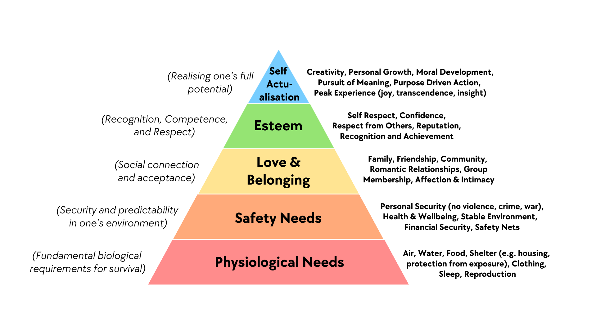
Excused lateness exceptions will be grounded in a policy where you can “pause” the class (due-date-wise, but also just, expectation-of-progress-wise more generally) to take the time you need to handle things happening in your life. Then, you can “resume” work once you feel more centered/once you find yourself back on stable ground. The “Maslow’s hierarchy” model from psychology (Figure 1) provides a straightforward way to think about this approach.
.png)
Learning about causal inference is way up there in the blue triangle, so, it’s important that you feel like the first four levels are solidified before you turn your focus back to classwork. And, it’s a win-win, because it means that once you’re back in action you can be more engaged and receptive to new topics, rather than being forced to “simulate” being in the blue triangle while in reality struggling in other spots!
References
Footnotes
Pearl (2000) represents a key work in this field of research, as it essentially brought together different pieces of causal models into one unified, rigorous framework.↩︎
Challenge yourself to keep watching to the end of the 5th video here, if you can! Even if you feel frustrated/scared! Because, the examples (e.g., macro vs. microeconomics) are what we mainly care about here, more so than e.g. the mathematical definition of entropy (which we will go towards at a slower pace!)↩︎