Week 8: Ecological Inference, Propensity Scores

DSAN 5650: Causal Inference for Computational Social Science
Summer 2026, Georgetown University

Author

Affiliation

Jeff Jacobs

jj1088@georgetown.edu

Open slides in new window →

Schedule

Today’s Planned Schedule:

	Start	End	Topic
Lecture	6:30pm	6:40pm	Final Project Pep Talk →
	6:40pm	7:15pm	Ecological Inference →
	7:15pm	8:00pm	Controlling For Things vs. Matching/Weighting →
Break!	8:00pm	8:10pm
	8:10pm	8:30pm	Propensity Score Lab →
	8:30pm	9:00pm	Causal Inferences with Text →

\[ \DeclareMathOperator*{\argmax}{argmax} \DeclareMathOperator*{\argmin}{argmin} \newcommand{\bigexp}[1]{\exp\mkern-4mu\left[ #1 \right]} \newcommand{\bigexpect}[1]{\mathbb{E}\mkern-4mu \left[ #1 \right]} \newcommand{\definedas}{\overset{\small\text{def}}{=}} \newcommand{\definedalign}{\overset{\phantom{\text{defn}}}{=}} \newcommand{\eqeventual}{\overset{\text{eventually}}{=}} \newcommand{\Err}{\text{Err}} \newcommand{\expect}[1]{\mathbb{E}[#1]} \newcommand{\expectsq}[1]{\mathbb{E}^2[#1]} \newcommand{\fw}[1]{\texttt{#1}} \newcommand{\given}{\mid} \newcommand{\green}[1]{\color{green}{#1}} \newcommand{\heads}{\outcome{heads}} \newcommand{\iid}{\overset{\text{\small{iid}}}{\sim}} \newcommand{\lik}{\mathcal{L}} \newcommand{\loglik}{\ell} \DeclareMathOperator*{\maximize}{maximize} \DeclareMathOperator*{\minimize}{minimize} \newcommand{\mle}{\textsf{ML}} \newcommand{\nimplies}{\;\not\!\!\!\!\implies} \newcommand{\orange}[1]{\color{orange}{#1}} \newcommand{\outcome}[1]{\textsf{#1}} \newcommand{\param}[1]{{\color{purple} #1}} \newcommand{\pgsamplespace}{\{\green{1},\green{2},\green{3},\purp{4},\purp{5},\purp{6}\}} \newcommand{\pedge}[2]{\require{enclose}\enclose{circle}{~{#1}~} \rightarrow \; \enclose{circle}{\kern.01em {#2}~\kern.01em}} \newcommand{\pnode}[1]{\require{enclose}\enclose{circle}{\kern.1em {#1} \kern.1em}} \newcommand{\ponode}[1]{\require{enclose}\enclose{box}[background=lightgray]{{#1}}} \newcommand{\pnodesp}[1]{\require{enclose}\enclose{circle}{~{#1}~}} \newcommand{\purp}[1]{\color{purple}{#1}} \newcommand{\sign}{\text{Sign}} \newcommand{\spacecap}{\; \cap \;} \newcommand{\spacewedge}{\; \wedge \;} \newcommand{\tails}{\outcome{tails}} \newcommand{\Var}[1]{\text{Var}[#1]} \newcommand{\bigVar}[1]{\text{Var}\mkern-4mu \left[ #1 \right]} \]

library(tidyverse)

── Attaching core tidyverse packages ──────────────────────── tidyverse 2.0.0 ──
✔ dplyr     1.1.4     ✔ readr     2.1.5
✔ forcats   1.0.0     ✔ stringr   1.5.1
✔ ggplot2   3.5.1     ✔ tibble    3.3.0
✔ lubridate 1.9.4     ✔ tidyr     1.3.1
✔ purrr     1.0.4     
── Conflicts ────────────────────────────────────────── tidyverse_conflicts() ──
✖ dplyr::filter() masks stats::filter()
✖ dplyr::lag()    masks stats::lag()
ℹ Use the conflicted package (<http://conflicted.r-lib.org/>) to force all conflicts to become errors

source("../dsan-globals/stat_binscatter.r")
source("../dsan-globals/_globals.r")

Final Projects

• Notion! Then, choose a path (rough draft of paths):
  • Modeling a social phenomenon with PGMs
  • Taking an existing project/interest (e.g., from 5300) and pushing towards the causality asymptote
• Choose a path by Tuesday, July 15, 6:30pm EDT

Ecological Inference (EI)

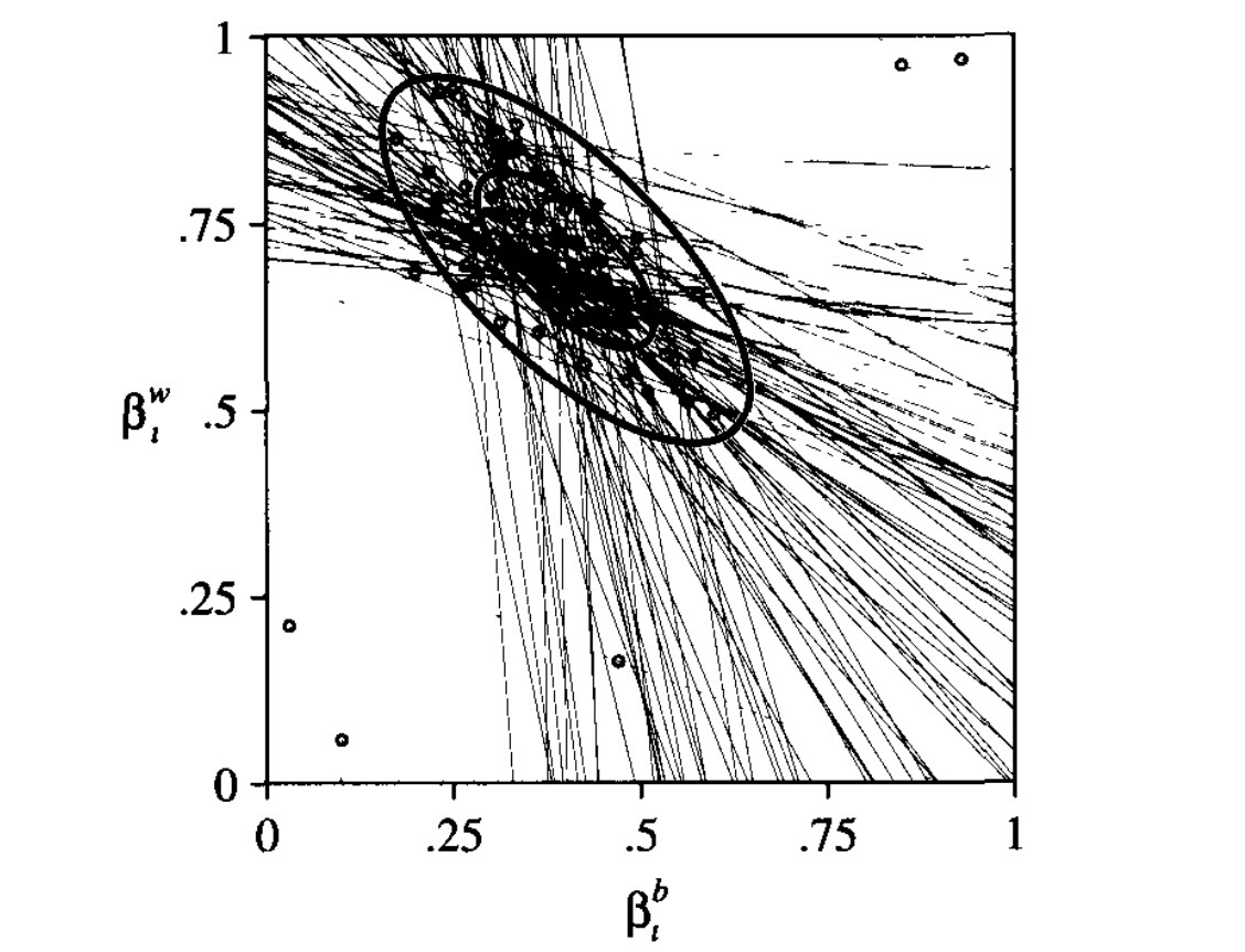
• Here, our priors will encode logical constraints (weakly-informative)
• Then, our statistical model will model probabilities of micro-level statistics subject to these constraints

potted_plant Here lines represent logical constraints on parameters, while the ellipses are contours of the probability distribution pooling this information

Logic = Probability Theory with \(\Pr(E) = 0\) or \(1\)

• Tomography Plot Demo

\(2 \times 2\) Setup

	Status
Vote Choice	Unemployed	Employed	Total
Nazis	\(W_{i1}\)	\(W_{i2}\)	\(Y_i\)
Other	\(1 - W_{i1}\)	\(1 - W_{i2}\)	\(1 - Y_i\)
Total	\(X_i\)	\(1 - X_i\)	\(1\)

Propensity Score Weighting

• HW1 matching: similarity either 1 (applied to same schools) or 0 (didn’t apply to same schools)
• Propensity scores: model quality of match
• \(\Rightarrow\) Opens up (literally) infinite possibilities between 0 and 1!
• \(\Rightarrow\) Use your unsupervised learning skills (matching via clustering)
• \(\Rightarrow\) Use your supervised learning skills (propensity scores = logistic regression coefficients!)

Figure 1: Should this be matched with an apple? Or an orange? Porque no los dos! [Image source]

• \(\Rightarrow\) Use your diagnostic skills: e.g., methods for evaluating clusters / preventing overfitting

Working Example: Growth Mindset(!)

• From Athey and Wager (2019)
• Treatment \(T\), called intervention in the dataset: a seminar on growth mindset for high school students
• Outcome \(Y\), called achievement_score in the dataset: performance on state’s standardized test
• In a perfect world, we could just compute

\[ \mathbb{E}[Y \mid T = 1] - \mathbb{E}[Y \mid T = 0] \]

library(tidyverse)
library(broom)
student_df <- read_csv("assets/learning_mindset.csv")

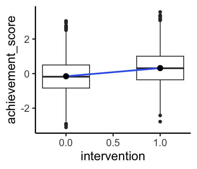
Rows: 10391 Columns: 13
── Column specification ────────────────────────────────────────────────────────
Delimiter: ","
dbl (13): schoolid, intervention, achievement_score, success_expect, ethnici...

ℹ Use `spec()` to retrieve the full column specification for this data.
ℹ Specify the column types or set `show_col_types = FALSE` to quiet this message.

(mean_df <- student_df |> group_by(intervention) |> summarize(mean_score=mean(achievement_score)))

intervention	mean_score
0	-0.1538030
1	0.3184686

student_naive_lm <- lm(achievement_score ~ intervention, data=student_df)
student_naive_lm |> broom::tidy() |> select(term, estimate)

term	estimate
(Intercept)	-0.1538030
intervention	0.4722717

student_df |>
  ggplot(aes(x=intervention, y=achievement_score)) +
  geom_boxplot(
    aes(group=intervention),
    width=0.5
  ) +
  geom_smooth(
    method='lm',
    formula='y ~ x',
    se=TRUE
  ) +
  geom_point(
    data=mean_df,
    aes(x=intervention, y=mean_score),
    size=3
  ) +
  theme_dsan(base_size=16)

The Problem: Pesky Covariates

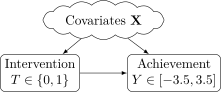
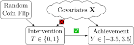
• Here the “blob” \(\mathbf{X}\) forms a fork, as drawn…
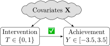
• But in reality the work of modeling is flying into the cloud and modeling the \(\mathbf{X}\)-\(T\) and \(\mathbf{X}\)-\(Y\) relationships (especially: figuring out which covariates \(X_j \in \mathbf{X}\) are colliders), so you can close the backdoors:

• This can be really difficult, for a bunch of reasons… What if there was an easier way?

If We Had Control Over Everything (Experiments vs. Observational Data Analysis)

• If we could intervene in the DGP, we could assign treatment randomly, thus removing the impact of Covariates on \(T\)!

• Alas, we are data scientists, not (necessarily) experiment-conductors, plus there are often ethical reasons to not perform experiments!
• …There’s still another approach!

Closing Backdoors the Too-Good-To-Be-True Way

• Key insight from causal thinking: Transformation of the problem from “control for all covariates” to “close all backdoor paths”…
• For the goal of just closing these paths, we have an alternative¹:

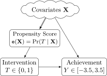
• Rosenbaum and Rubin (1983): there exists a statistic \(\mathtt{e}(\mathbf{X}) = \Pr(T \mid \mathbf{X})\), the propensity score, which “captures” info in \(\textbf{X}\) relevant to \(T\) such that
• Conditioning on \(\mathtt{e}(\mathbf{X})\) closes \(\mathbf{X} \Rightarrow \mathtt{e}(\mathbf{X}) \rightarrow T\) (\(\mathtt{e}(\mathbf{X})\) is a pipe)

• This would close backdoor path \(T \leftarrow \mathtt{e}(\mathbf{X}) \Leftarrow \mathbf{X} \rightarrow Y\), leaving only direct effect \(T \rightarrow Y\)! There’s one remaining complication…

Closing Backdoors via Propensity Score Estimation

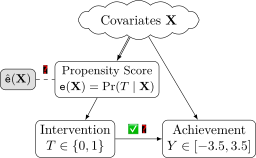
• Sadly we don’t observe true probability of being treated for all possible values of \(\mathbf{X}\)
• But, we can derive an estimate \(\hat{\mathtt{e}}(\mathbf{X})\) using our machine learning skills 😎
• We now have that \(\hat{\mathtt{e}}(\mathbf{X})\), as a proxy relative to the pipe \(\mathbf{X} \Rightarrow \mathtt{e}(\mathbf{X}) \rightarrow T\), blocks the pipe to the extent that it captures the true probability \(\mathtt{e}(\mathbf{X}) = \Pr(T \mid \mathbf{X})\)

• Backdoor Path: \(T \leftarrow \mathtt{e}(\mathbf{X}) \Leftarrow \mathbf{X} \rightarrow Y\)
• Closed in proportion to \(\left[ \text{Cor}(\hat{\mathtt{e}}(\mathbf{X}), \mathtt{e}(\mathbf{X})) \right]^2 = ❓\)

Sometimes-Helpful Thought Experiment

• Back in our basic confounding scenario:
• If there was only one covariate (\(\mathbf{X} = X\)), and it was a constant (\(\Pr(X = c) = 1\)), then all the variation in \(Y\) would be due to variation in \(T\)
• Less extreme: if person \(i\) has covariates \(\mathbf{X}_i\) and person \(j\) has covariates \(\mathbf{X}_j\), but \(\mathbf{X}_i = \mathbf{X}_j\), then variation in their outcomes is due solely to \(T\)

• Part of the logic of propensity score is that, if person \(i\) has covariates \(\mathbf{X}_i\) and person \(j\) has covariates \(\mathbf{X}_j\), but \(\mathtt{e}(\mathbf{X}_i) = \mathtt{e}(\mathbf{X}_j)\), then \(i\) and \(j\) are perfectly matched
• \(\Rightarrow\) (by fun math proof) variation in their outcomes is due solely to \(T\)

References

Athey, Susan, and Stefan Wager. 2019. “Estimating Treatment Effects with Causal Forests: An Application.” Pre-published February 20. https://doi.org/10.48550/arXiv.1902.07409.

Rosenbaum, Paul R., and Donald B. Rubin. 1983. “The Central Role of the Propensity Score in Observational Studies for Causal Effects.” Biometrika 70 (1): 41–55. https://doi.org/10.2307/2335942.

Footnotes

1. For reasons we’ll see later (double-robustness), you should ultimately try to achieve both goals!