Code
source("../dsan-globals/_globals.r")DSAN 5650: Causal Inference for Computational Social Science
Summer 2026, Georgetown University
Today’s Planned Schedule:
| Start | End | Topic | |
|---|---|---|---|
| Lecture | 6:30pm | 7:10pm | PGM as Modeling Language → |
| 7:10pm | 7:30pm | The Ladder of Causal Inference → | |
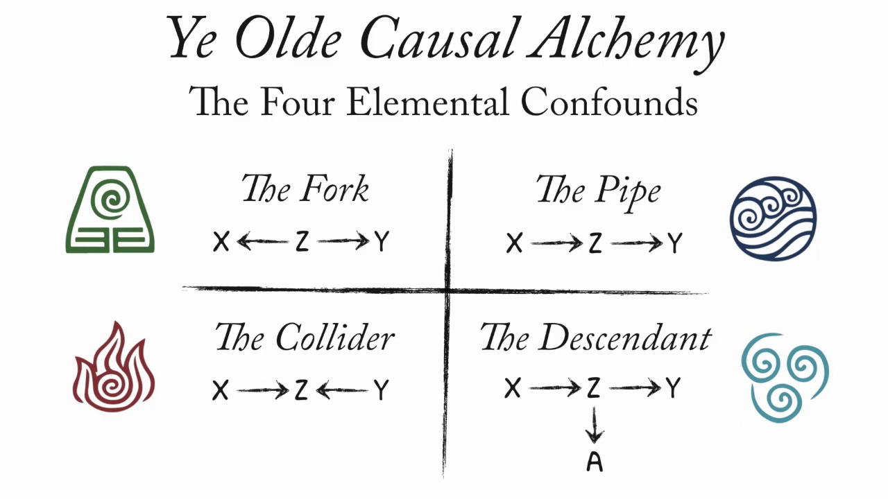
| 7:30pm | 7:50pm | Elemental Confounds I: Forks and Chains → | |
| Break! | 7:50pm | 8:00pm | |
| 8:00pm | 8:50pm | Elemental Confounds II: ⚠️Colliders⚠️ → | |
| 8:50pm | 9:00pm | Elemental Confounds III: Proxies → |
\[ \DeclareMathOperator*{\argmax}{argmax} \DeclareMathOperator*{\argmin}{argmin} \newcommand{\bigexp}[1]{\exp\mkern-4mu\left[ #1 \right]} \newcommand{\bigexpect}[1]{\mathbb{E}\mkern-4mu \left[ #1 \right]} \newcommand{\definedas}{\overset{\small\text{def}}{=}} \newcommand{\definedalign}{\overset{\phantom{\text{defn}}}{=}} \newcommand{\eqeventual}{\overset{\text{eventually}}{=}} \newcommand{\Err}{\text{Err}} \newcommand{\expect}[1]{\mathbb{E}[#1]} \newcommand{\expectsq}[1]{\mathbb{E}^2[#1]} \newcommand{\fw}[1]{\texttt{#1}} \newcommand{\given}{\mid} \newcommand{\green}[1]{\color{green}{#1}} \newcommand{\heads}{\outcome{heads}} \newcommand{\iid}{\overset{\text{\small{iid}}}{\sim}} \newcommand{\lik}{\mathcal{L}} \newcommand{\loglik}{\ell} \DeclareMathOperator*{\maximize}{maximize} \DeclareMathOperator*{\minimize}{minimize} \newcommand{\mle}{\textsf{ML}} \newcommand{\nimplies}{\;\not\!\!\!\!\implies} \newcommand{\orange}[1]{\color{orange}{#1}} \newcommand{\outcome}[1]{\textsf{#1}} \newcommand{\param}[1]{{\color{purple} #1}} \newcommand{\pgsamplespace}{\{\green{1},\green{2},\green{3},\purp{4},\purp{5},\purp{6}\}} \newcommand{\pedge}[2]{\require{enclose}\enclose{circle}{~{#1}~} \rightarrow \; \enclose{circle}{\kern.01em {#2}~\kern.01em}} \newcommand{\pnode}[1]{\require{enclose}\enclose{circle}{\kern.1em {#1} \kern.1em}} \newcommand{\ponode}[1]{\require{enclose}\enclose{box}[background=lightgray]{{#1}}} \newcommand{\pnodesp}[1]{\require{enclose}\enclose{circle}{~{#1}~}} \newcommand{\purp}[1]{\color{purple}{#1}} \newcommand{\sign}{\text{Sign}} \newcommand{\spacecap}{\; \cap \;} \newcommand{\spacewedge}{\; \wedge \;} \newcommand{\tails}{\outcome{tails}} \newcommand{\Var}[1]{\text{Var}[#1]} \newcommand{\bigVar}[1]{\text{Var}\mkern-4mu \left[ #1 \right]} \]
source("../dsan-globals/_globals.r")5300 → Now
Now → August: Class splits into two themes, running in parallel!

Languages give us a syntax…
| S | \(\rightarrow\) | NP VP |
| NP | \(\rightarrow\) | DetP N | AdjP NP |
| VP | \(\rightarrow\) | V NP |
| AdjP | \(\rightarrow\) | Adj | Adv AdjP |
| N | \(\rightarrow\) | frog | tadpole |
| V | \(\rightarrow\) | sees | likes |
| Adj | \(\rightarrow\) | big | small |
| Adv | \(\rightarrow\) | very |
| DetP | \(\rightarrow\) | a | the |
…For expressing arbitrary (infinitely many!) sentences

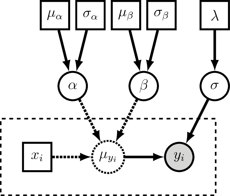
Need a language that can communicate the following info to estimation algorithm:

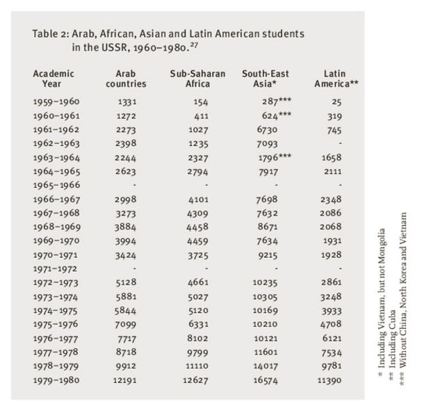
"Congo", "DRC", "Republic of Congo") can then be contextualized: can “track” and link data appropriately despite splits, merges, name changes| Entity | Data from 1947-1971 at... | Data from 1971-Present at... | ||
|---|---|---|---|---|
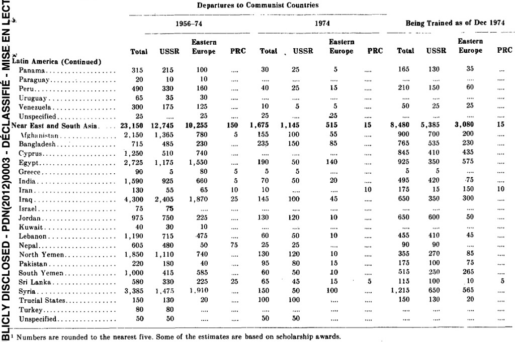
| \(\textsf{Pakistan}_{1979}\) | National Level: | \(\frac{62}{62+70} \times\) “Pakistan” | National Level: | “Pakistan” |
| Subnational Level: | “West Pakistan” | Subnational Level: | \(\sum_{i \in \text{Regions}}\text{data}_i\) | |
| \(\textsf{Bangladesh}_{1979}\) | National Level: | \(\frac{70}{62+70} \times\) “Pakistan” | National Level: | “Bangladesh” |
| Subnational Level: | “East Pakistan” | Subnational Level: | \(\sum_{i \in \text{Regions}}\text{data}_i\) | |
 |
Counterfactuals: What would have happened, if history was slightly different… \(\Pr(Y_{M=M_0} \mid \textsf{do}(X)) - \Pr(Y_{M=M_0} \mid \textsf{do}(\neg X))\) |
||||
 |
Intervention: What happens if I… \(\Pr(Y \mid \textsf{do}(X)) - \Pr(Y \mid \textsf{do}(\neg X))\) |
||||
 |
Association: What happened? \(\Pr(Y \mid X) - \Pr(Y \mid \neg X)\) |
||||
library(tidyverse) # For ggplot── Attaching core tidyverse packages ──────────────────────── tidyverse 2.0.0 ──
✔ dplyr 1.2.1 ✔ readr 2.2.0
✔ forcats 1.0.1 ✔ stringr 1.6.0
✔ lubridate 1.9.5 ✔ tibble 3.3.1
✔ purrr 1.2.1 ✔ tidyr 1.3.2
── Conflicts ────────────────────────────────────────── tidyverse_conflicts() ──
✖ dplyr::filter() masks stats::filter()
✖ dplyr::lag() masks stats::lag()
ℹ Use the conflicted package (<http://conflicted.r-lib.org/>) to force all conflicts to become errorslibrary(extraDistr) # For rbern()
Attaching package: 'extraDistr'

The following object is masked from 'package:purrr':

rduniflibrary(patchwork) # For side-by-side plotting
library(ggtext) # For colors in titles
library(rethinking)Loading required package: cmdstanr
This is cmdstanr version 0.9.0
- CmdStanR documentation and vignettes: mc-stan.org/cmdstanr
- CmdStan path: /Users/jpj/.cmdstan/cmdstan-2.36.0
- CmdStan version: 2.36.0
A newer version of CmdStan is available. See ?install_cmdstan() to install it.
To disable this check set option or environment variable cmdstanr_no_ver_check=TRUE.
Loading required package: posterior
This is posterior version 1.7.0
Attaching package: 'posterior'
The following objects are masked from 'package:stats':
mad, sd, var
The following objects are masked from 'package:base':
%in%, match
Loading required package: parallel
rethinking (Version 2.42)
Attaching package: 'rethinking'
The following objects are masked from 'package:extraDistr':
dbern, dlaplace, dpareto, rbern, rlaplace, rpareto
The following object is masked from 'package:purrr':
map
The following object is masked from 'package:stats':
rstudentlibrary(dagitty)
n_d <- 10000 # For discrete RVs
n_c <- 300 # For continuous RVslibrary(rethinking)
library(dagitty)
library(ggdag)
source("mydrawdag.r")
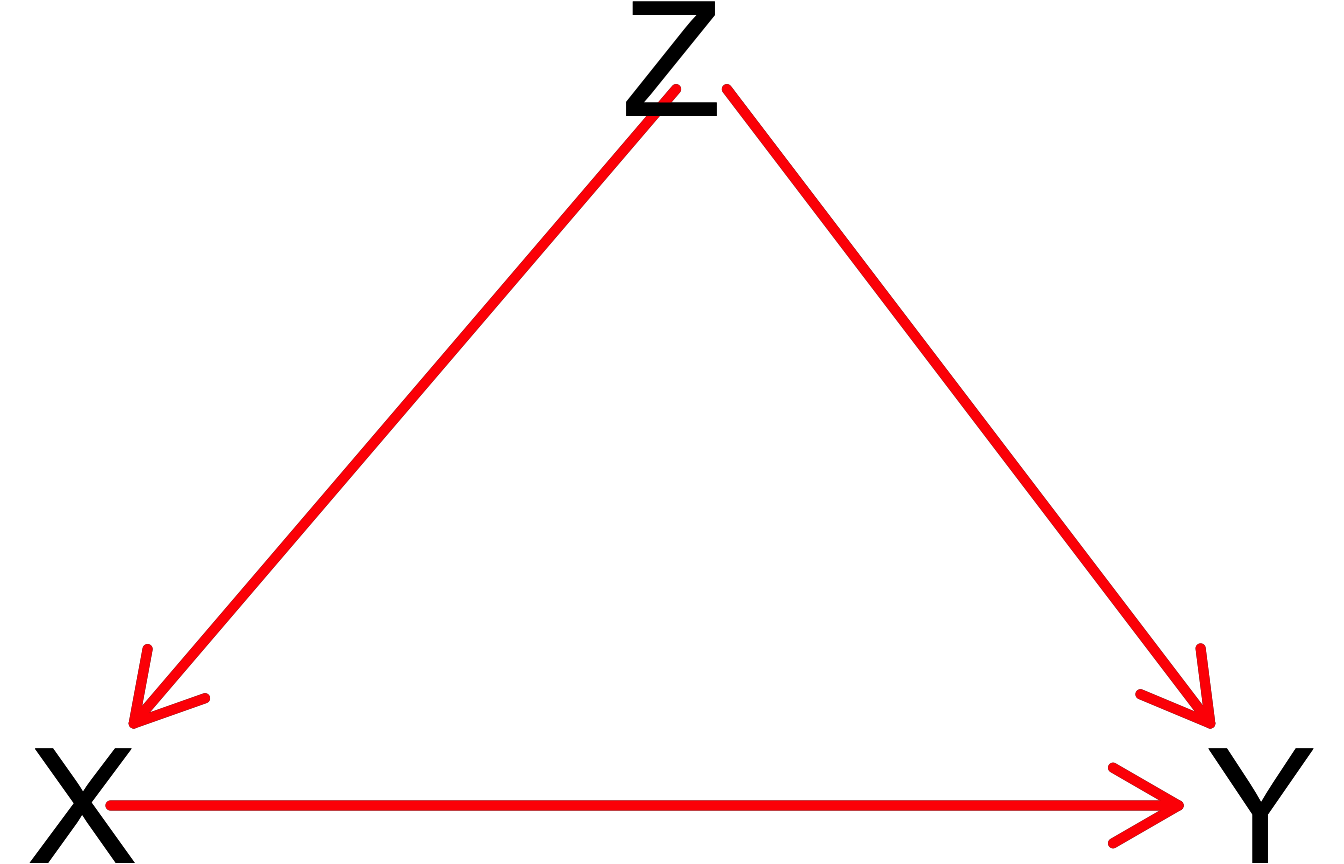
pipe_dag <- dagitty("dag{
X[exposure]
Y[outcome]
X -> Y
X -> Z
Z -> Y
}")
coordinates(pipe_dag) <- list(
x=c(X=0, Z=0.5, Y=1),
y=c(X=1, Z=0.5, Y=1)
)
drawdag_jj(
pipe_dag, cex=5, lwd=5,
)
drawopenpaths_jj(
pipe_dag, cex=5, lwd=5,
)
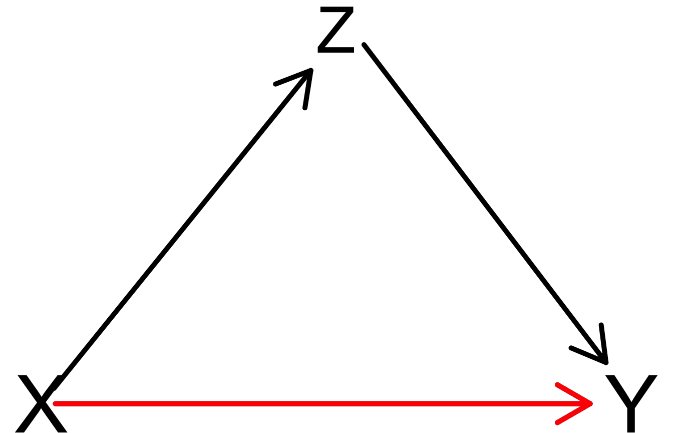
adj_sets <- adjustmentSets(
pipe_dag, effect="direct"
)
writeLines("Adjustment sets (direct effect):")
adj_sets
set.seed(5650)
cpipe_df <- tibble(
X = rnorm(n_c),
Z = rbern(n_c, plogis(X)),
Y = rnorm(n_c, 2 * Z - 1)
)
cpipe_lm <- lm(Y ~ X, data=cpipe_df)
cpipe_slope <- round(cpipe_lm$coef['X'], 3)
cpipe_z0_lm <- lm(Y ~ X, data=cpipe_df |> filter(Z == 0))
cpipe_z0_slope <- round(cpipe_z0_lm$coef['X'], 2)
cpipe_z0_label <- paste0("<span style='color: #e69f00;'>Slope<sub>Z=0</sub> = ",cpipe_z0_slope,"</span>")
cpipe_z1_lm <- lm(Y ~ X, data=cpipe_df |> filter(Z == 1))
cpipe_z1_slope <- round(cpipe_z1_lm$coef['X'], 2)
cpipe_z1_label <- paste0("<span style='color: #56b4e9;'>Slope<sub>Z=1</sub> = ",cpipe_z1_slope,"</span>")
cpipe_z_texlabel <- paste0(cpipe_z0_label, " | ", cpipe_z1_label)
cpipe_xmin <- min(cpipe_df$X)
cpipe_xmax <- max(cpipe_df$X)
ggplot() +
# Points
geom_point(
data=cpipe_df |> filter(Y > -3),
aes(x=X, y=Y, color=factor(Z)),
size=0.4*g_pointsize,
alpha=0.8
) +
# Overall lm
geom_smooth(
data=cpipe_df, aes(x=X, y=Y),
method = lm, se = FALSE,
linewidth = 2.75, color='white'
) +
geom_smooth(
data=cpipe_df, aes(x=X, y=Y),
method = lm, se = FALSE,
linewidth = 2, color='black'
) +
theme_dsan(base_size=18) +
theme(
plot.title = element_text(size=18),
plot.subtitle = element_markdown(size=16)
) +
# coord_equal() +
labs(
title = paste0(
"Unstratified Slope = ",cpipe_slope
),
x = "X", y = "Y", color = "Z"
)

Attaching package: 'ggdag'The following object is masked from 'package:stats':
filter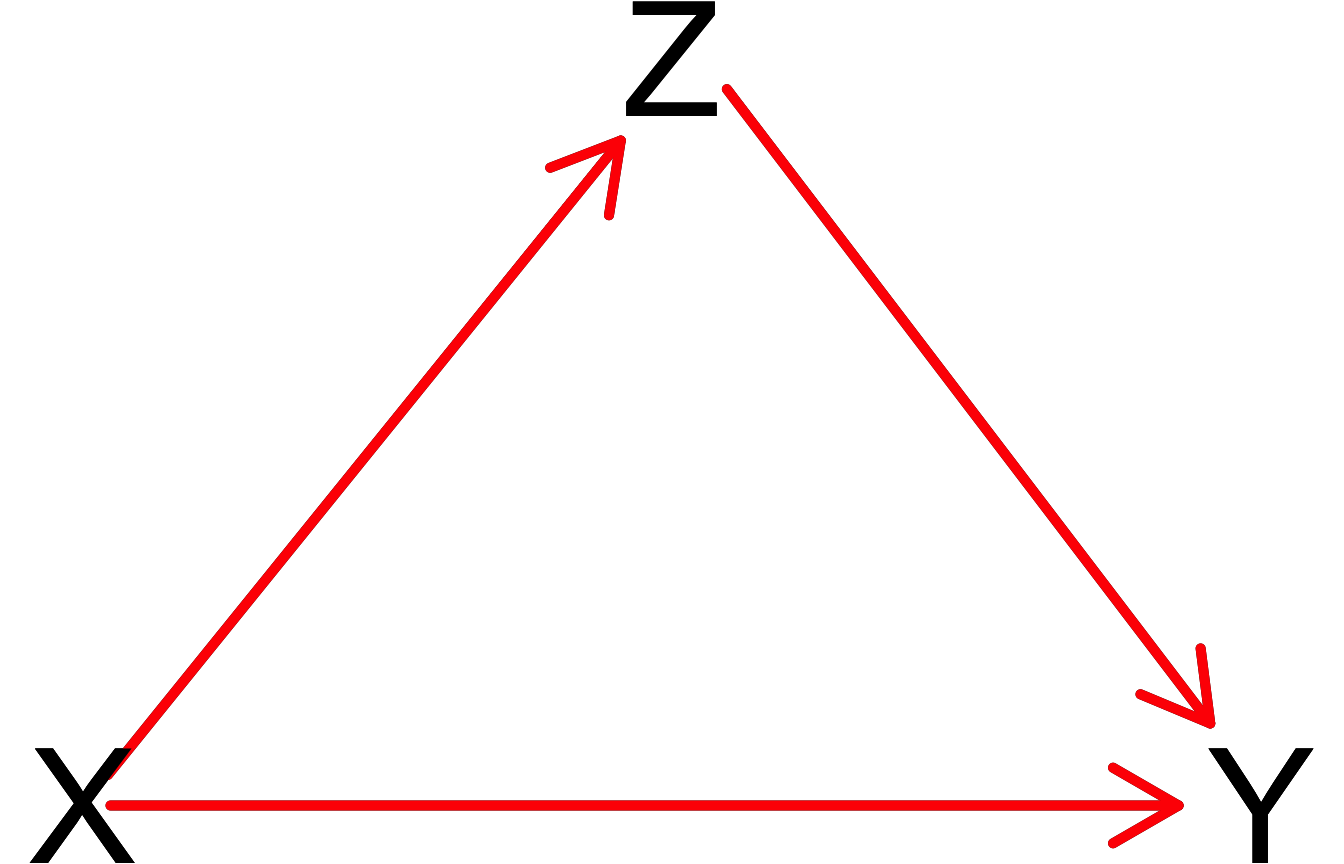
Adjustment sets (direct effect):
{ Z }
`geom_smooth()` using formula = 'y ~ x'
`geom_smooth()` using formula = 'y ~ x'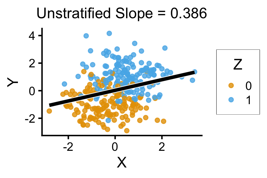
library(rethinking)
library(dagitty)
library(ggdag)
pipe_dag_closed <-dagitty("dag{
X[exposure]
Y[outcome]
Z[adjustedNode]
X -> Y
X -> Z
Z -> Y
}")
coordinates(pipe_dag_closed) <- list(
x=c(X=0, Z=0.5, Y=1),
y=c(X=1, Z=0.5, Y=1)
)
drawdag_jj(
pipe_dag_closed, cex=4, lwd=5, radius=10
)
drawopenpaths_jj(
pipe_dag_closed, Z="Z", lwd=5
)
adj_sets_closed <- adjustmentSets(
pipe_dag_closed
)
writeLines("Adjustment sets (direct effect):")
adj_sets_closed
set.seed(5650)
cpipe_df <- tibble(
X = rnorm(n_c),
Z = rbern(n_c, plogis(X)),
Y = rnorm(n_c, 2 * Z - 1)
)
cpipe_lm <- lm(Y ~ X, data=cpipe_df)
cpipe_slope <- round(cpipe_lm$coef['X'], 3)
cpipe_z0_lm <- lm(Y ~ X, data=cpipe_df |> filter(Z == 0))
cpipe_z0_slope <- round(cpipe_z0_lm$coef['X'], 2)
cpipe_z0_label <- paste0("<span style='color: #e69f00;'>Slope<sub>Z=0</sub> = ",cpipe_z0_slope,"</span>")
cpipe_z1_lm <- lm(Y ~ X, data=cpipe_df |> filter(Z == 1))
cpipe_z1_slope <- round(cpipe_z1_lm$coef['X'], 2)
cpipe_z1_label <- paste0("<span style='color: #56b4e9;'>Slope<sub>Z=1</sub> = ",cpipe_z1_slope,"</span>")
cpipe_z_texlabel <- paste0(cpipe_z0_label, " | ", cpipe_z1_label)
cpipe_xmin <- min(cpipe_df$X)
cpipe_xmax <- max(cpipe_df$X)
ggplot() +
# Points
geom_point(
data=cpipe_df |> filter(Y > -3),
aes(x=X, y=Y, color=factor(Z)),
size=0.4*g_pointsize,
alpha=0.8
) +
# geom_smooth(
# data=cpipe_df, aes(x=X, y=Y),
# method = lm, se = FALSE,
# linewidth = 2.75, color='white'
# ) +
# geom_smooth(
# data=cpipe_df, aes(x=X, y=Y),
# method = lm, se = FALSE,
# linewidth = 2, color='black'
# ) +
# Stratified lm
# (slightly larger black lines)
geom_smooth(
data=cpipe_df,
aes(x=X, y=Y, group=factor(Z)),
method=lm, se=FALSE, fullrange=TRUE,
linewidth=2.75, color='black'
) +
# (Colored lines)
geom_smooth(
data=cpipe_df,
aes(x=X, y=Y, color=factor(Z)),
method=lm, se=FALSE, fullrange=TRUE,
linewidth=2
) +
theme_dsan(base_size=18) +
theme(
plot.title = element_markdown(size=18),
plot.subtitle = element_markdown(size=16)
) +
# coord_equal() +
labs(
title=cpipe_z_texlabel,
x = "X", y = "Y", color = "Z"
)

Adjustment sets (direct effect):
{}`geom_smooth()` using formula = 'y ~ x'
`geom_smooth()` using formula = 'y ~ x'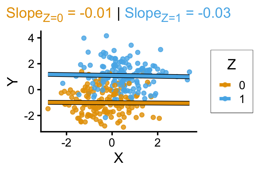
library(rethinking)
library(dagitty)
library(ggdag)
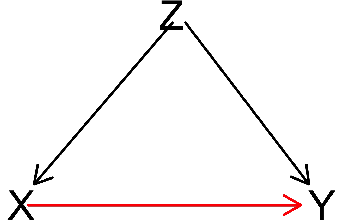
pipe_dag <-dagitty("dag{
X[exposure]
Y[outcome]
X -> Y
Z -> X
Z -> Y
}")
coordinates(pipe_dag) <- list(
x=c(X=0, Z=0.5, Y=1),
y=c(X=1, Z=0.5, Y=1)
)
drawdag_jj(pipe_dag, cex=5, lwd=5)
drawopenpaths_jj(pipe_dag, cex=5, lwd=5)
adj_sets <- adjustmentSets(
pipe_dag, effect="direct"
)
writeLines("Adjustment sets (direct effect):")
adj_sets
library(ggtext)
set.seed(5650)
cfork_df <- tibble(
Z = rbern(n_c),
X = rnorm(n_c, 2 * Z - 1),
Y = rnorm(n_c, 2 * Z - 1)
)
library(latex2exp)
overall_lm <- lm(Y ~ X, data=cfork_df)
overall_slope <- round(overall_lm$coef['X'], 3)
z0_lm <- lm(Y ~ X, data=cfork_df |> filter(Z == 0))
z0_slope <- round(z0_lm$coef['X'], 2)
z0_label <- paste0("<span style='color: #e69f00;'>Slope<sub>Z=0</sub> = ",z0_slope,"</span>")
z1_lm <- lm(Y ~ X, data=cfork_df |> filter(Z == 1))
z1_slope <- round(z1_lm$coef['X'], 2)
z1_label <- paste0("<span style='color: #56b4e9;'>Slope<sub>Z=1</sub> = ",z1_slope,"</span>")
z_texlabel <- paste0(z0_label, " | ", z1_label)
cfork_xmin <- min(cfork_df$X)
cfork_xmax <- max(cfork_df$X)
ggplot() +
# Points
geom_point(
data=cfork_df,
aes(x=X, y=Y, color=factor(Z)),
size=0.4*g_pointsize,
alpha=0.8
) +
# Overall lm
geom_smooth(
data=cfork_df, aes(x=X, y=Y),
method = lm, se = FALSE,
linewidth = 2.75, color='white'
) +
geom_smooth(
data=cfork_df, aes(x=X, y=Y),
method = lm, se = FALSE,
linewidth = 2, color='black'
) +
theme_dsan(base_size=18) +
theme(
plot.title = element_text(size=18),
plot.subtitle = element_markdown(size=16)
) +
# coord_equal() +
labs(
title = paste0(
"Unstratified Slope = ",overall_slope
),
x = "X", y = "Y", color = "Z"
)

Adjustment sets (direct effect):
{ Z }`geom_smooth()` using formula = 'y ~ x'
`geom_smooth()` using formula = 'y ~ x'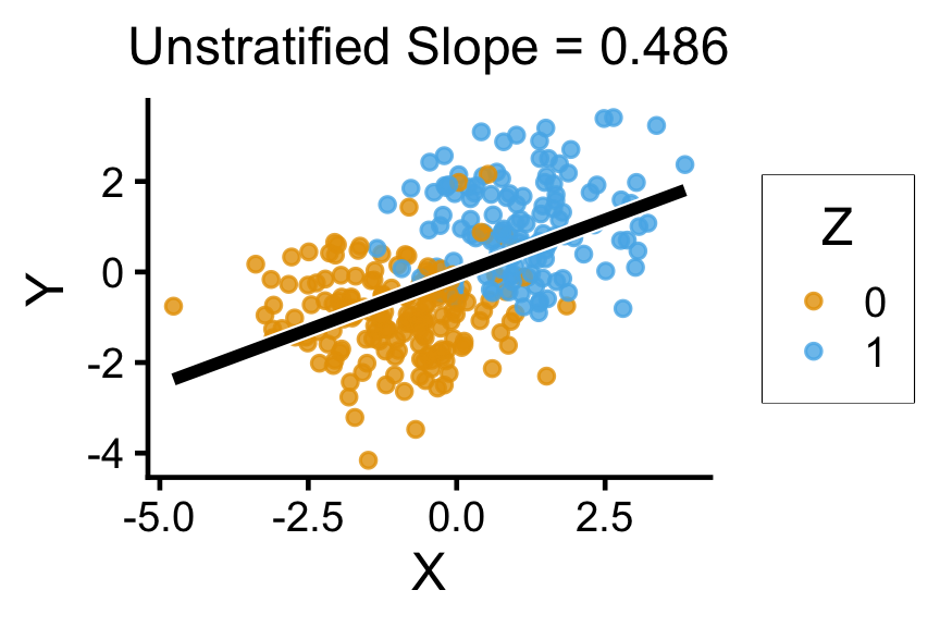
fork_dag_closed <-dagitty("dag{
X[exposure]
Y[outcome]
Z[adjustedNode]
X -> Y
Z -> X
Z -> Y
}")
coordinates(fork_dag_closed) <- list(
x=c(X=0, Z=0.5, Y=1),
y=c(X=1, Z=0.5, Y=1)
)
fork_dag_closed <- setVariableStatus(
fork_dag_closed, "adjustedNode", "Z"
)
drawdag_jj(
fork_dag_closed, cex=5, lwd=5
)
drawopenpaths_jj(
fork_dag_closed, Z="Z", lwd=5
)
library(ggtext)
set.seed(5650)
cfork_df <- tibble(
Z = rbern(n_c),
X = rnorm(n_c, 2 * Z - 1),
Y = rnorm(n_c, 2 * Z - 1)
)
library(latex2exp)
overall_lm <- lm(Y ~ X, data=cfork_df)
overall_slope <- round(overall_lm$coef['X'], 3)
z0_lm <- lm(Y ~ X, data=cfork_df |> filter(Z == 0))
z0_slope <- round(z0_lm$coef['X'], 2)
z0_label <- paste0("<span style='color: #e69f00;'>Slope<sub>Z=0</sub> = ",z0_slope,"</span>")
z1_lm <- lm(Y ~ X, data=cfork_df |> filter(Z == 1))
z1_slope <- round(z1_lm$coef['X'], 2)
z1_label <- paste0("<span style='color: #56b4e9;'>Slope<sub>Z=1</sub> = ",z1_slope,"</span>")
z_texlabel <- paste0(z0_label, " | ", z1_label)
cfork_xmin <- min(cfork_df$X)
cfork_xmax <- max(cfork_df$X)
ggplot() +
# Points
geom_point(
data=cfork_df,
aes(x=X, y=Y, color=factor(Z)),
size=0.4*g_pointsize,
alpha=0.8
) +
# Overall lm
# geom_smooth(
# data=cfork_df, aes(x=X, y=Y),
# method = lm, se = FALSE,
# linewidth = 2.75, color='white'
# ) +
# geom_smooth(
# data=cfork_df, aes(x=X, y=Y),
# method = lm, se = FALSE,
# linewidth = 2, color='black'
# ) +
# Stratified lm
# (slightly larger black lines)
geom_smooth(
data=cfork_df,
aes(x=X, y=Y, group=factor(Z)),
method=lm, se=FALSE, fullrange=TRUE,
linewidth=2.75, color='black'
) +
# (Colored lines)
geom_smooth(
data=cfork_df,
aes(x=X, y=Y, color=factor(Z)),
method=lm, se=FALSE, fullrange=TRUE,
linewidth=2
) +
theme_dsan(base_size=18) +
theme(
plot.title = element_text(size=18),
plot.subtitle = element_markdown(size=16)
) +
# coord_equal() +
labs(
# title = paste0(
# "Unstratified Slope = ",overall_slope
# ),
# subtitle=z_texlabel,
subtitle=z_texlabel,
x = "X", y = "Y", color = "Z"
)

`geom_smooth()` using formula = 'y ~ x'
`geom_smooth()` using formula = 'y ~ x'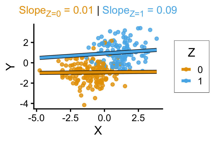

library(tidyverse)
library(extraDistr)
library(latex2exp)
set.seed(5650)
cprox_df <- tibble(
X = rnorm(n_c),
Z = rbern(n_c, plogis(X)),
Y = rnorm(n_c, 2 * Z - 1),
A = rbern(n_c, (1-Z)*0.86 + Z*0.14)
)
cprox_lm <- lm(Y ~ X, data=cprox_df)
cprox_slope <- round(cprox_lm$coef['X'], 3)
cprox_a0_lm <- lm(Y ~ X, data=cprox_df |> filter(A == 0))
cprox_a0_slope <- round(cprox_a0_lm$coef['X'], 2)
cprox_a0_label <- paste0("<span style='color: #e69f00;'>Slope<sub>Z=0</sub> = ",cprox_a0_slope,"</span>")
# A == 1 lm
cprox_a1_lm <- lm(Y ~ X, data=cprox_df |> filter(A == 1))
cprox_a1_slope <- round(cprox_a1_lm$coef['X'], 2)
cprox_a1_label <- paste0("<span style='color: #56b4e9;'>Slope<sub>Z=1</sub> = ",cprox_a1_slope,"</span>")
cprox_a_texlabel <- paste0(cprox_a0_label, " | ", cprox_a1_label)
cprox_xmin <- min(cprox_df$X)
cprox_xmax <- max(cprox_df$X)
ggplot() +
# Points
geom_point(
data=cprox_df |> filter(Y > -3),
aes(x=X, y=Y, color=factor(A)),
size=0.5*g_pointsize,
alpha=0.8
) +
# Overall lm
geom_smooth(
data=cprox_df, aes(x=X, y=Y),
method = lm, se = FALSE,
linewidth = 2.5, color='black'
) +
# Stratified lm
# (slightly larger black lines)
geom_smooth(
data=cprox_df,
aes(x=X, y=Y, group=factor(A)),
method=lm, se=FALSE, fullrange=TRUE,
linewidth=2.75, color='black'
) +
# (Colored lines)
geom_smooth(
data=cprox_df,
aes(x=X, y=Y, color=factor(A)),
method=lm, se=FALSE, fullrange=TRUE,
linewidth=2
) +
theme_dsan(base_size=20) +
theme(
plot.title = element_text(size=20),
plot.subtitle = element_markdown(size=18)
) +
# coord_equal() +
labs(
title = paste0(
"Unstratified Slope = ",cprox_slope
),
subtitle=cprox_a_texlabel,
x = "X", y = "Y", color = "A"
)`geom_smooth()` using formula = 'y ~ x'
`geom_smooth()` using formula = 'y ~ x'
`geom_smooth()` using formula = 'y ~ x'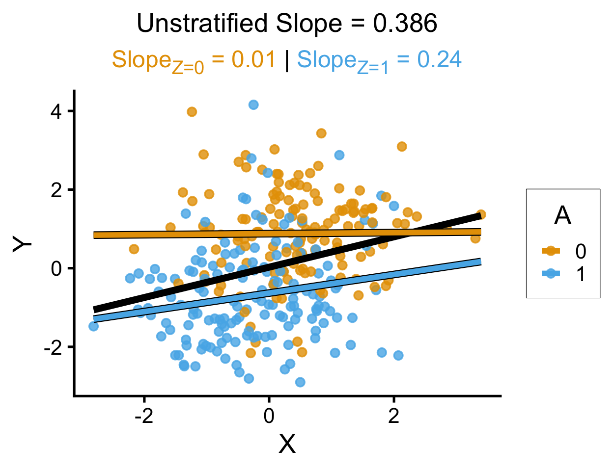
library(rethinking)
library(dagitty)
library(ggdag)
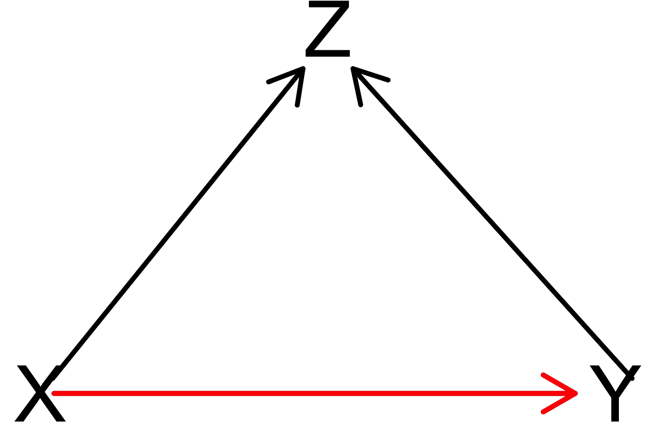
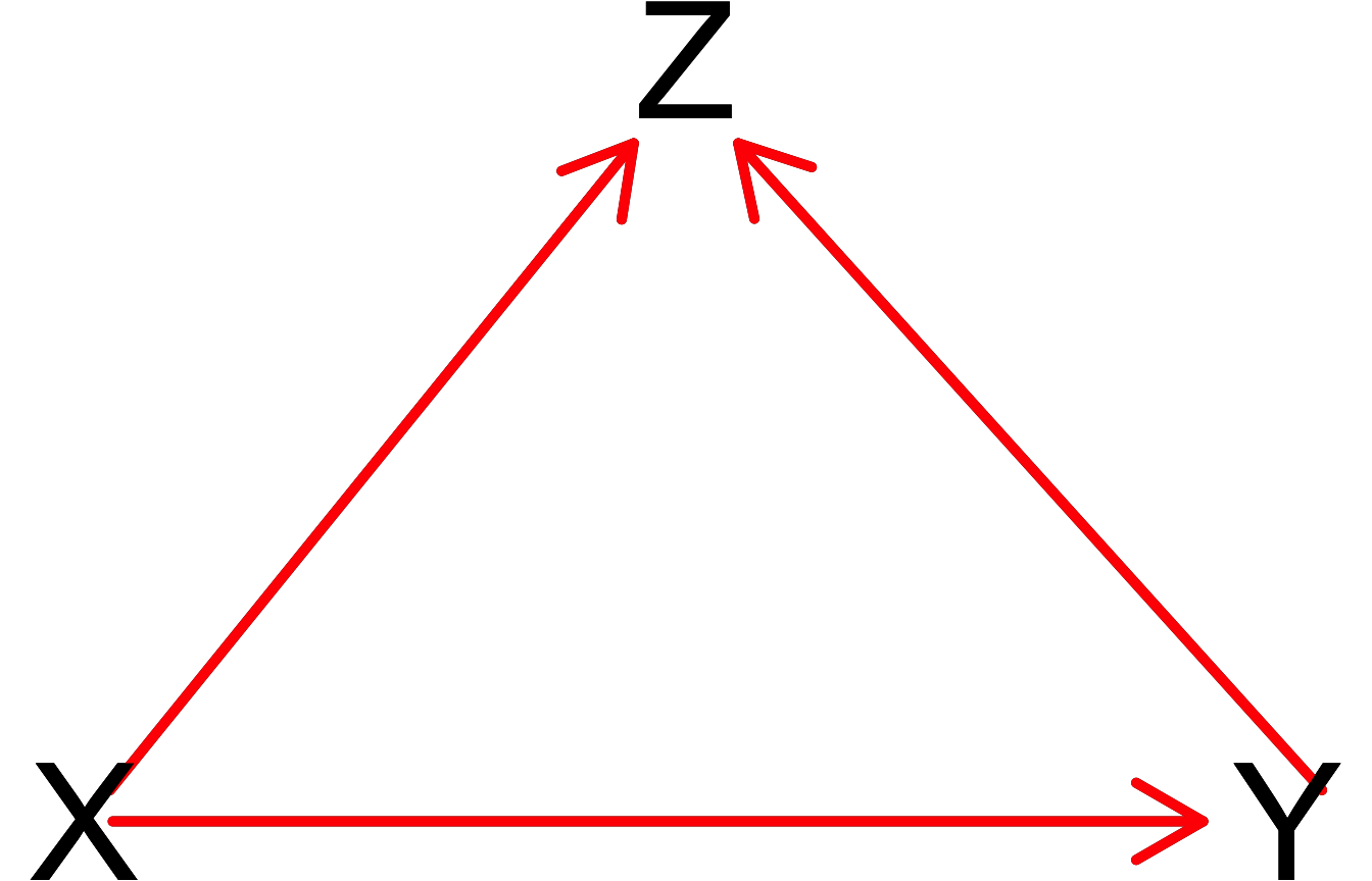
coll_dag <-dagitty("dag{
X[exposure]
Y[outcome]
X -> Y
X -> Z
Y -> Z
}")
coordinates(coll_dag) <- list(
x=c(X=0, Z=0.5, Y=1),
y=c(X=1, Z=0.5, Y=1)
)
drawdag_jj(
coll_dag, cex=5, lwd=5
)
drawopenpaths_jj(coll_dag, lwd=5)
adj_sets_coll <- adjustmentSets(
coll_dag, effect="direct"
)
writeLines("Adjustment sets (direct effect):")
adj_sets_coll
set.seed(5650)
ccoll_df <- tibble(
X = rnorm(n_c),
Y = rnorm(n_c),
Z = rbern(n_c, plogis(2 * (X + Y - 1)))
)
ccoll_lm <- lm(Y ~ X, data=ccoll_df)
ccoll_slope <- round(ccoll_lm$coef['X'], 3)
ccoll_z0_lm <- lm(Y ~ X, data=ccoll_df |> filter(Z == 0))
ccoll_z0_slope <- round(ccoll_z0_lm$coef['X'], 2)
ccoll_z0_label <- paste0("<span style='color: #e69f00;'>Slope<sub>Z=0</sub> = ",ccoll_z0_slope,"</span>")
ccoll_z1_lm <- lm(Y ~ X, data=ccoll_df |> filter(Z == 1))
ccoll_z1_slope <- round(ccoll_z1_lm$coef['X'], 2)
ccoll_z1_label <- paste0("<span style='color: #56b4e9;'>Slope<sub>Z=1</sub> = ",ccoll_z1_slope,"</span>")
ccoll_z_texlabel <- paste0(ccoll_z0_label, " | ", ccoll_z1_label)
ccoll_xmin <- min(ccoll_df$X)
ccoll_xmax <- max(ccoll_df$X)
ggplot() +
# Points
geom_point(
data=ccoll_df |> filter(Y > -3),
aes(x=X, y=Y, color=factor(Z)),
size=0.4*g_pointsize,
alpha=0.8
) +
# Overall lm
geom_smooth(
data=ccoll_df, aes(x=X, y=Y),
method = lm, se = FALSE,
linewidth = 2.75, color='white'
) +
geom_smooth(
data=ccoll_df, aes(x=X, y=Y),
method = lm, se = FALSE,
linewidth = 2, color='black'
) +
theme_dsan(base_size=18) +
theme(
plot.title = element_markdown(size=18),
plot.subtitle = element_markdown(size=16)
) +
# coord_equal() +
labs(
# title=ccoll_z_texlabel,
title=paste0("Unstratified Slope = ",ccoll_slope),
x = "X", y = "Y", color = "Z"
)

Adjustment sets (direct effect):
{}
`geom_smooth()` using formula = 'y ~ x'
`geom_smooth()` using formula = 'y ~ x'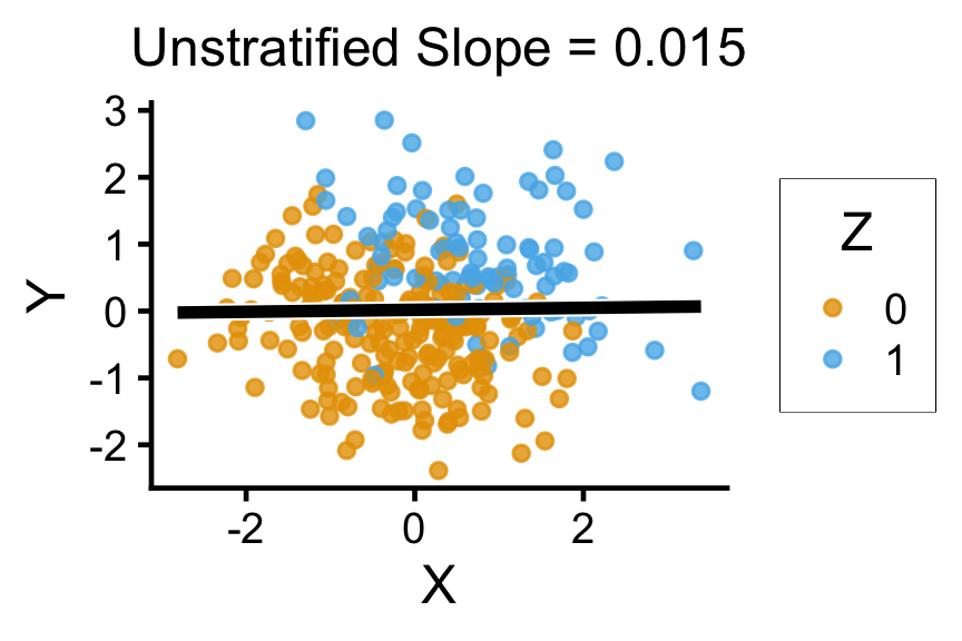
library(rethinking)
library(dagitty)
library(ggdag)
fork_dag_closed <- dagitty("dag{
X[exposure]
Y[outcome]
Z[adjustedNode]
X -> Y
X -> Z
Y -> Z
}")
coordinates(fork_dag_closed) <- list(
x=c(X=0, Z=0.5, Y=1),
y=c(X=1, Z=0.5, Y=1)
)
fork_dag_closed <- setVariableStatus(
fork_dag_closed, "adjustedNode", "Z"
)
drawdag_jj(
fork_dag_closed,
cex=5, lwd=5,
)
drawopenpaths_jj(
fork_dag_closed, Z="Z", lwd=5
)
set.seed(5650)
ccoll_df <- tibble(
X = rnorm(n_c),
Y = rnorm(n_c),
Z = rbern(n_c, plogis(2 * (X + Y - 1)))
)
ccoll_lm <- lm(Y ~ X, data=ccoll_df)
ccoll_slope <- round(ccoll_lm$coef['X'], 3)
ccoll_z0_lm <- lm(Y ~ X, data=ccoll_df |> filter(Z == 0))
ccoll_z0_slope <- round(ccoll_z0_lm$coef['X'], 2)
ccoll_z0_label <- paste0("<span style='color: #e69f00;'>Slope<sub>Z=0</sub> = ",ccoll_z0_slope,"</span>")
ccoll_z1_lm <- lm(Y ~ X, data=ccoll_df |> filter(Z == 1))
ccoll_z1_slope <- round(ccoll_z1_lm$coef['X'], 2)
ccoll_z1_label <- paste0("<span style='color: #56b4e9;'>Slope<sub>Z=1</sub> = ",ccoll_z1_slope,"</span>")
ccoll_z_texlabel <- paste0(ccoll_z0_label, " | ", ccoll_z1_label)
ccoll_xmin <- min(ccoll_df$X)
ccoll_xmax <- max(ccoll_df$X)
ggplot() +
# Points
geom_point(
data=ccoll_df |> filter(Y > -3),
aes(x=X, y=Y, color=factor(Z)),
size=0.4*g_pointsize,
alpha=0.8
) +
# Stratified lm
# (slightly larger black lines)
geom_smooth(
data=ccoll_df,
aes(x=X, y=Y, group=factor(Z)),
method=lm, se=FALSE, fullrange=TRUE,
linewidth=2.75, color='black'
) +
# (Colored lines)
geom_smooth(
data=ccoll_df,
aes(x=X, y=Y, color=factor(Z)),
method=lm, se=FALSE, fullrange=TRUE,
linewidth=2
) +
theme_dsan(base_size=18) +
theme(
plot.title = element_markdown(size=18),
plot.subtitle = element_markdown(size=16)
) +
# coord_equal() +
labs(
title=ccoll_z_texlabel,
x = "X", y = "Y", color = "Z"
)


`geom_smooth()` using formula = 'y ~ x'
`geom_smooth()` using formula = 'y ~ x'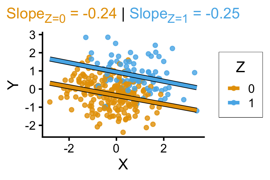
set.seed(5650)
grant_df <- tibble(
newsworthy = runif(n_c, 0, 10),
rigorous = runif(n_c, 0, 10),
awarded = ifelse(newsworthy + rigorous > 10, 1, 0)
)
grant_lm <- lm(rigorous ~ newsworthy, data=grant_df)
grant_slope <- round(grant_lm$coef['newsworthy'], 3)
grant_z0_lm <- lm(rigorous ~ newsworthy, data=grant_df |> filter(awarded == 0))
grant_z0_slope <- round(grant_z0_lm$coef['newsworthy'], 2)
grant_z1_lm <- lm(rigorous ~ newsworthy, data=grant_df |> filter(awarded == 1))
grant_z1_slope <- round(grant_z1_lm$coef['newsworthy'], 2)
grant_z1_label <- paste0("<span style='color: #56b4e9;'>Slope<sub>+</sub> = ",grant_z1_slope,"</span>")
grant_z_texlabel <- grant_z1_label
grant_xmin <- min(grant_df$newsworthy)
grant_xmax <- max(grant_df$newsworthy)
ggplot() +
# Points
geom_point(
data=grant_df |> filter(rigorous > -3),
aes(x=newsworthy, y=rigorous, color=factor(awarded)),
size=0.4*g_pointsize,
alpha=0.8
) +
# Stratified lm
# (slightly larger black lines)
geom_smooth(
data=grant_df |> filter(awarded == 1),
aes(x=newsworthy, y=rigorous, group=factor(awarded)),
method=lm, se=FALSE, fullrange=TRUE,
linewidth=2.75, color='black'
) +
# (Colored lines)
geom_smooth(
data=grant_df |> filter(awarded == 1),
aes(x=newsworthy, y=rigorous, color=factor(awarded)),
method=lm, se=FALSE, fullrange=TRUE,
linewidth=2
) +
theme_dsan(base_size=18) +
theme(
plot.title = element_markdown(size=18),
plot.subtitle = element_markdown(size=16)
) +
coord_equal() +
labs(
title=grant_z_texlabel,
x = "Newsworthy?", y = "Rigorous?", color = "awarded"
)
set.seed(5650)
grant_df <- tibble(
newsworthy = rnorm(n_c, 5, 1),
rigorous = rnorm(n_c, 5, 1),
awarded = ifelse(newsworthy + rigorous > 12, 1, 0)
)
grant_lm <- lm(rigorous ~ newsworthy, data=grant_df)
grant_slope <- round(grant_lm$coef['newsworthy'], 3)
grant_z0_lm <- lm(rigorous ~ newsworthy, data=grant_df |> filter(awarded == 0))
grant_z0_slope <- round(grant_z0_lm$coef['newsworthy'], 2)
grant_z1_lm <- lm(rigorous ~ newsworthy, data=grant_df |> filter(awarded == 1))
grant_z1_slope <- round(grant_z1_lm$coef['newsworthy'], 2)
grant_z1_label <- paste0("<span style='color: #56b4e9;'>Slope<sub>+</sub> = ",grant_z1_slope,"</span>")
grant_z_texlabel <- grant_z1_label
grant_xmin <- min(grant_df$newsworthy)
grant_xmax <- max(grant_df$newsworthy)
ggplot() +
# Points
geom_point(
data=grant_df |> filter(rigorous > -3),
aes(x=newsworthy, y=rigorous, color=factor(awarded)),
size=0.35*g_pointsize,
alpha=0.8
) +
# Stratified lm
# (slightly larger black lines)
geom_smooth(
data=grant_df |> filter(awarded == 1),
aes(x=newsworthy, y=rigorous, group=factor(awarded)),
method=lm, se=FALSE, fullrange=TRUE,
linewidth=2.75, color='black'
) +
# (Colored lines)
geom_smooth(
data=grant_df |> filter(awarded == 1),
aes(x=newsworthy, y=rigorous, color=factor(awarded)),
method=lm, se=FALSE, fullrange=TRUE,
linewidth=2
) +
theme_dsan(base_size=18) +
theme(
plot.title = element_markdown(size=18),
plot.subtitle = element_markdown(size=16)
) +
coord_equal() +
labs(
title=grant_z_texlabel,
x = "Newsworthy?", y = "Rigorous?", color = "awarded"
)`geom_smooth()` using formula = 'y ~ x'
`geom_smooth()` using formula = 'y ~ x'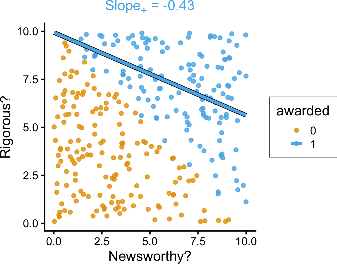
`geom_smooth()` using formula = 'y ~ x'
`geom_smooth()` using formula = 'y ~ x'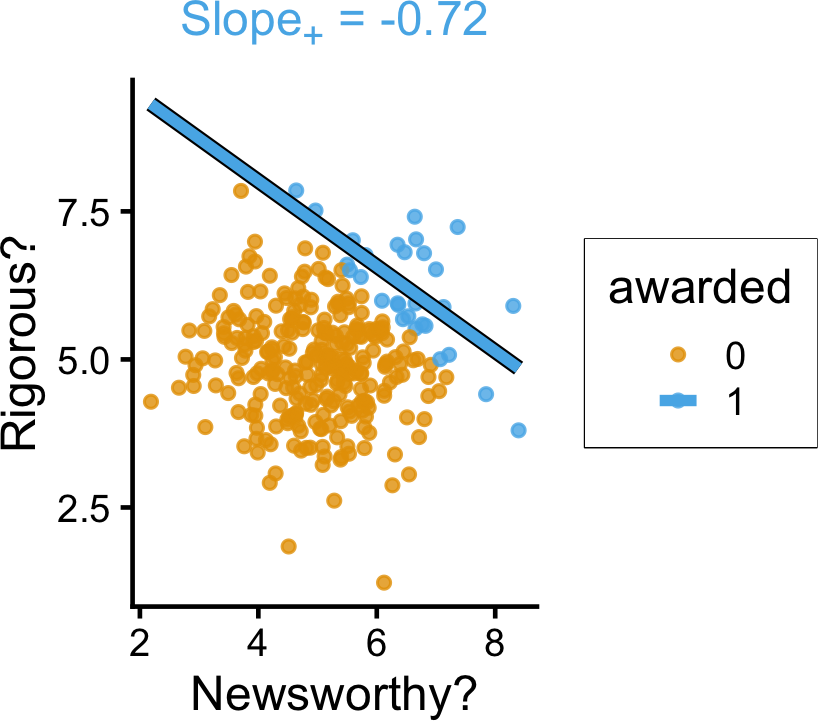
Helpful metaphor (Gleijeses 2013): Cuba \(\approx\) Forward-deployed “3rd World Outpost” for USSR (Soviet $ but Cuban training of PAIGC → MPLA), as Israel \(\approx\) Forward-deployed “3rd World Outpost” for US (US $ but Israeli training of SAVAK → SADF)↩︎