Week 4: Clearing the Path from Cause to Effect
DSAN 5650: Causal Inference for Computational Social Science
Summer 2026, Georgetown University
Wednesday, June 10, 2026
Roadmap
5300 → Now
- In e.g. 5300, you learned a bunch of ad hoc models: Linear Regression, Decision Trees, SVMs
- PGMs provide a formalized modeling language for “writing out” models unambiguously in a way your computer understands: specifying exactly how to estimate parameters from data
Now → August: Class splits into two themes, running in parallel!
- What kinds of cool comp social sci models are unlocked, that we can now implement in this language? [HW2]
- How can we expand PGM vocabulary to incorporate causality? [Midterm]

Why Take the Time to Learn a Modeling Language (vs. Individual Models)?
- My answer: allows you to adapt to specifics/idiosyncrasies of your problem!
- Language metaphor: Learning models vs. learning modeling language \(\Leftrightarrow\) Learning phrases in a language vs. learning to speak the language
- “Hello, one hamburger please” is good, but what if you…
- Are allergic to ketchup and need to make sure it’s removed
- Want to replace sesame seed bun with poppy seed bun, if they have it
- Prefer spicy, but not too spicy, mustard Bun only Animal style …
Languages give us a syntax…
| S | \(\rightarrow\) | NP VP |
| NP | \(\rightarrow\) | DetP N | AdjP NP |
| VP | \(\rightarrow\) | V NP |
| AdjP | \(\rightarrow\) | Adj | Adv AdjP |
| N | \(\rightarrow\) | frog | tadpole |
| V | \(\rightarrow\) | sees | likes |
| Adj | \(\rightarrow\) | big | small |
| Adv | \(\rightarrow\) | very |
| DetP | \(\rightarrow\) | a | the |
…For expressing arbitrary (infinitely many!) sentences

Example 1: Multilevel Tadpoles (McElreath, Ch. 13)
Need a language that can communicate the following info to estimation algorithm:
- Unit of observation is tadpole, but unit of analysis is tank
- Ultimately, I care about \(Y =\) survival rate (dependent var), as function of \(X =\) tank properties (independent var)
- …But the \(n_i = 48\) tanks actually come in \(n_j = 3\) types: small (10 bois), medium (25), large (35) (Bonus: What if there are different numbers of tanks per type?)
- I need it to account for impact of tank size, then pool info across tank sizes

From McElreath (2020)
Example 2: Dissertation Nightmare

The Ladder of Causal Inference
 |
Counterfactuals: What would have happened, if history was slightly different… \(\Pr(Y_{M=M_0} \mid \textsf{do}(X)) - \Pr(Y_{M=M_0} \mid \textsf{do}(\neg X))\) |
||||
 |
Intervention: What happens if I… \(\Pr(Y \mid \textsf{do}(X)) - \Pr(Y \mid \textsf{do}(\neg X))\) |
||||
 |
Association: What happened? \(\Pr(Y \mid X) - \Pr(Y \mid \neg X)\) |
||||
- \(\leadsto\) Stuff we add to probability theory in 5650 is to combat confounding: to “fix” whatever is making \(\Pr(Y \mid X) \neq \Pr(Y \mid \textsf{do}(X))\)!
The Four Elemental Confounds
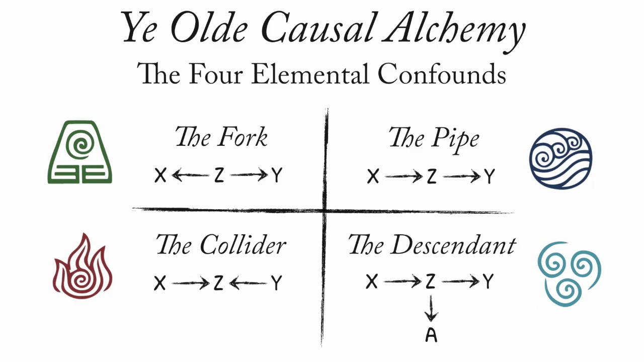
From Richard McElreath’s Statistical Rethinking Lectures
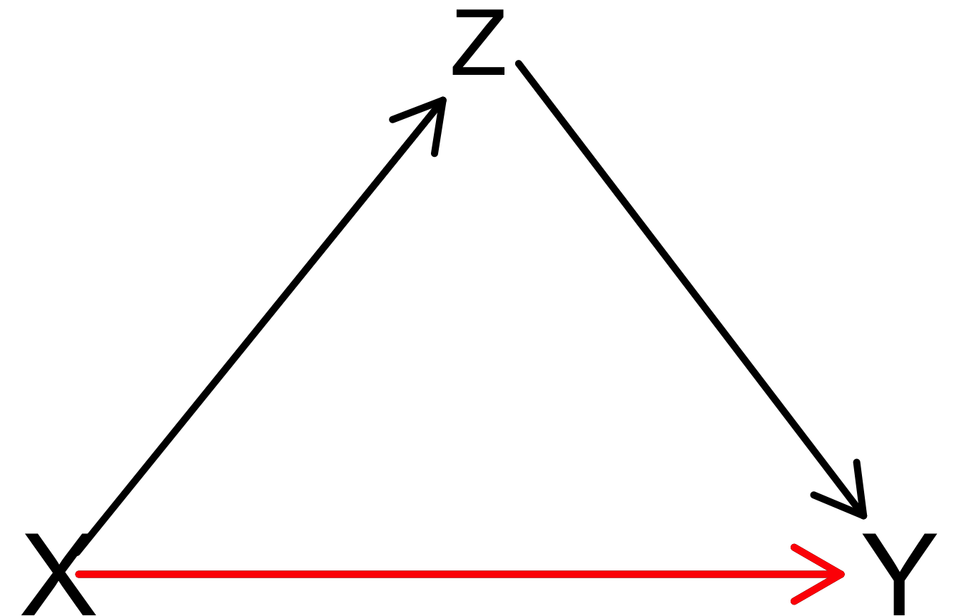
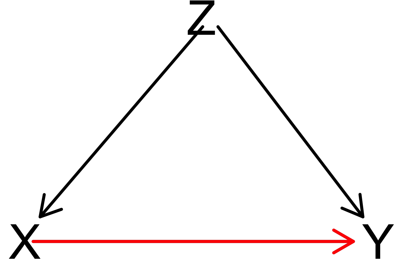
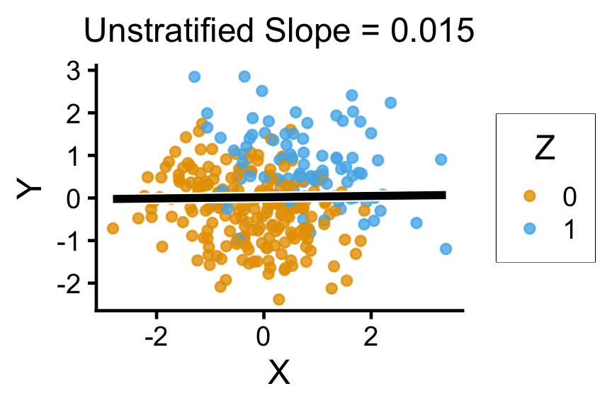
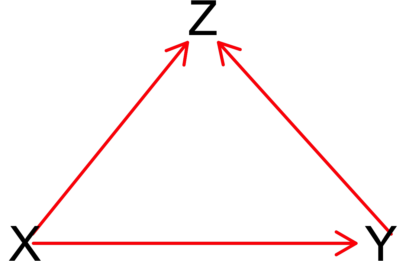
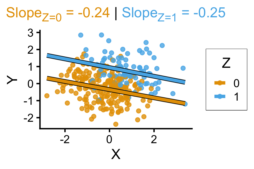
Pipes \(X \rightarrow Z \rightarrow Y\): Conditioning = Blocking
Code
library(rethinking)
library(dagitty)
library(ggdag)
source("mydrawdag.r")
pipe_dag <- dagitty("dag{
X[exposure]
Y[outcome]
X -> Y
X -> Z
Z -> Y
}")
coordinates(pipe_dag) <- list(
x=c(X=0, Z=0.5, Y=1),
y=c(X=1, Z=0.5, Y=1)
)
drawdag_jj(
pipe_dag, cex=5, lwd=5,
)
drawopenpaths_jj(
pipe_dag, cex=5, lwd=5,
)
adj_sets <- adjustmentSets(
pipe_dag, effect="direct"
)
writeLines("Adjustment sets (direct effect):")
adj_sets
set.seed(5650)
cpipe_df <- tibble(
X = rnorm(n_c),
Z = rbern(n_c, plogis(X)),
Y = rnorm(n_c, 2 * Z - 1)
)
cpipe_lm <- lm(Y ~ X, data=cpipe_df)
cpipe_slope <- round(cpipe_lm$coef['X'], 3)
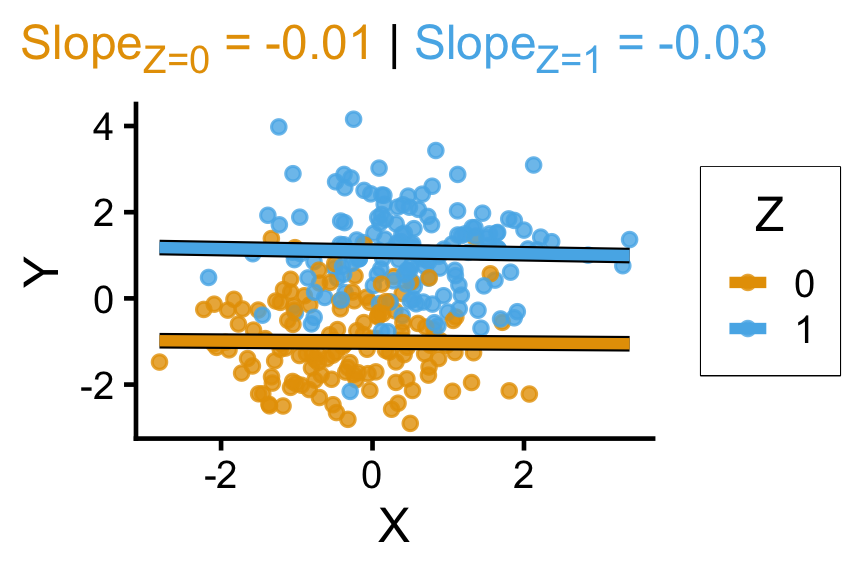
cpipe_z0_lm <- lm(Y ~ X, data=cpipe_df |> filter(Z == 0))
cpipe_z0_slope <- round(cpipe_z0_lm$coef['X'], 2)
cpipe_z0_label <- paste0("<span style='color: #e69f00;'>Slope<sub>Z=0</sub> = ",cpipe_z0_slope,"</span>")
cpipe_z1_lm <- lm(Y ~ X, data=cpipe_df |> filter(Z == 1))
cpipe_z1_slope <- round(cpipe_z1_lm$coef['X'], 2)
cpipe_z1_label <- paste0("<span style='color: #56b4e9;'>Slope<sub>Z=1</sub> = ",cpipe_z1_slope,"</span>")
cpipe_z_texlabel <- paste0(cpipe_z0_label, " | ", cpipe_z1_label)
cpipe_xmin <- min(cpipe_df$X)
cpipe_xmax <- max(cpipe_df$X)
ggplot() +
# Points
geom_point(
data=cpipe_df |> filter(Y > -3),
aes(x=X, y=Y, color=factor(Z)),
size=0.4*g_pointsize,
alpha=0.8
) +
# Overall lm
geom_smooth(
data=cpipe_df, aes(x=X, y=Y),
method = lm, se = FALSE,
linewidth = 2.75, color='white'
) +
geom_smooth(
data=cpipe_df, aes(x=X, y=Y),
method = lm, se = FALSE,
linewidth = 2, color='black'
) +
theme_dsan(base_size=18) +
theme(
plot.title = element_text(size=18),
plot.subtitle = element_markdown(size=16)
) +
# coord_equal() +
labs(
title = paste0(
"Unstratified Slope = ",cpipe_slope
),
x = "X", y = "Y", color = "Z"
)

Adjustment sets (direct effect):
{ Z }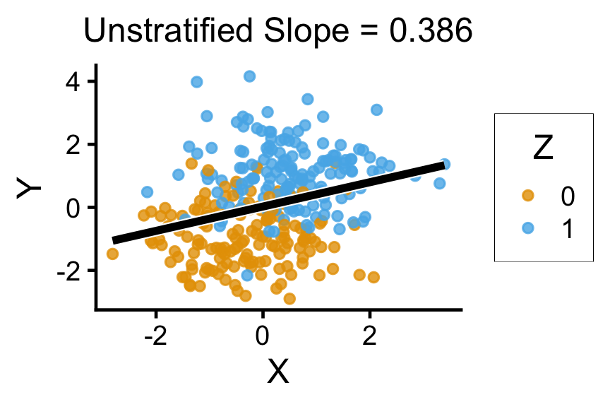
Code
library(rethinking)
library(dagitty)
library(ggdag)
pipe_dag_closed <-dagitty("dag{
X[exposure]
Y[outcome]
Z[adjustedNode]
X -> Y
X -> Z
Z -> Y
}")
coordinates(pipe_dag_closed) <- list(
    x=c(X=0, Z=0.5, Y=1),
    y=c(X=1, Z=0.5, Y=1)
)
drawdag_jj(
  pipe_dag_closed, cex=4, lwd=5, radius=10
)
drawopenpaths_jj(
  pipe_dag_closed, Z="Z", lwd=5
)
adj_sets_closed <- adjustmentSets(
    pipe_dag_closed
)
writeLines("Adjustment sets (direct effect):")
adj_sets_closed
set.seed(5650)
cpipe_df <- tibble(
    X = rnorm(n_c),
    Z = rbern(n_c, plogis(X)),
    Y = rnorm(n_c, 2 * Z - 1)
)
cpipe_lm <- lm(Y ~ X, data=cpipe_df)
cpipe_slope <- round(cpipe_lm$coef['X'], 3)
cpipe_z0_lm <- lm(Y ~ X, data=cpipe_df |> filter(Z == 0))
cpipe_z0_slope <- round(cpipe_z0_lm$coef['X'], 2)
cpipe_z0_label <- paste0("<span style='color: #e69f00;'>Slope<sub>Z=0</sub> = ",cpipe_z0_slope,"</span>")
cpipe_z1_lm <- lm(Y ~ X, data=cpipe_df |> filter(Z == 1))
cpipe_z1_slope <- round(cpipe_z1_lm$coef['X'], 2)
cpipe_z1_label <- paste0("<span style='color: #56b4e9;'>Slope<sub>Z=1</sub> = ",cpipe_z1_slope,"</span>")
cpipe_z_texlabel <- paste0(cpipe_z0_label, " | ", cpipe_z1_label)
cpipe_xmin <- min(cpipe_df$X)
cpipe_xmax <- max(cpipe_df$X)
ggplot() +
  # Points
  geom_point(
    data=cpipe_df |> filter(Y > -3),
    aes(x=X, y=Y, color=factor(Z)),
    size=0.4*g_pointsize,
    alpha=0.8
  ) +
  # geom_smooth(
  #   data=cpipe_df, aes(x=X, y=Y),
  #   method = lm, se = FALSE,
  #   linewidth = 2.75, color='white'
  # ) +
  # geom_smooth(
  #   data=cpipe_df, aes(x=X, y=Y),
  #   method = lm, se = FALSE,
  #   linewidth = 2, color='black'
  # ) +
  # Stratified lm
  # (slightly larger black lines)
  geom_smooth(
    data=cpipe_df,
    aes(x=X, y=Y, group=factor(Z)),
    method=lm, se=FALSE, fullrange=TRUE,
    linewidth=2.75, color='black'
  ) +
  # (Colored lines)
  geom_smooth(
    data=cpipe_df,
    aes(x=X, y=Y, color=factor(Z)),
    method=lm, se=FALSE, fullrange=TRUE,
    linewidth=2
  ) +
  theme_dsan(base_size=18) +
  theme(
    plot.title = element_markdown(size=18),
    plot.subtitle = element_markdown(size=16)
  ) +
  # coord_equal() +
  labs(
    title=cpipe_z_texlabel,
    x = "X", y = "Y", color = "Z"
  )

Adjustment sets (direct effect):
{}
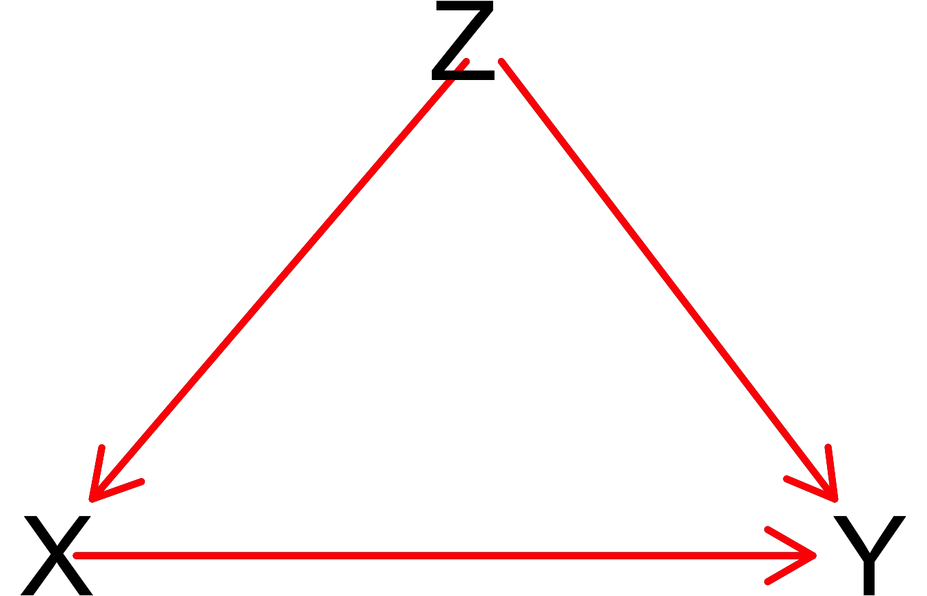
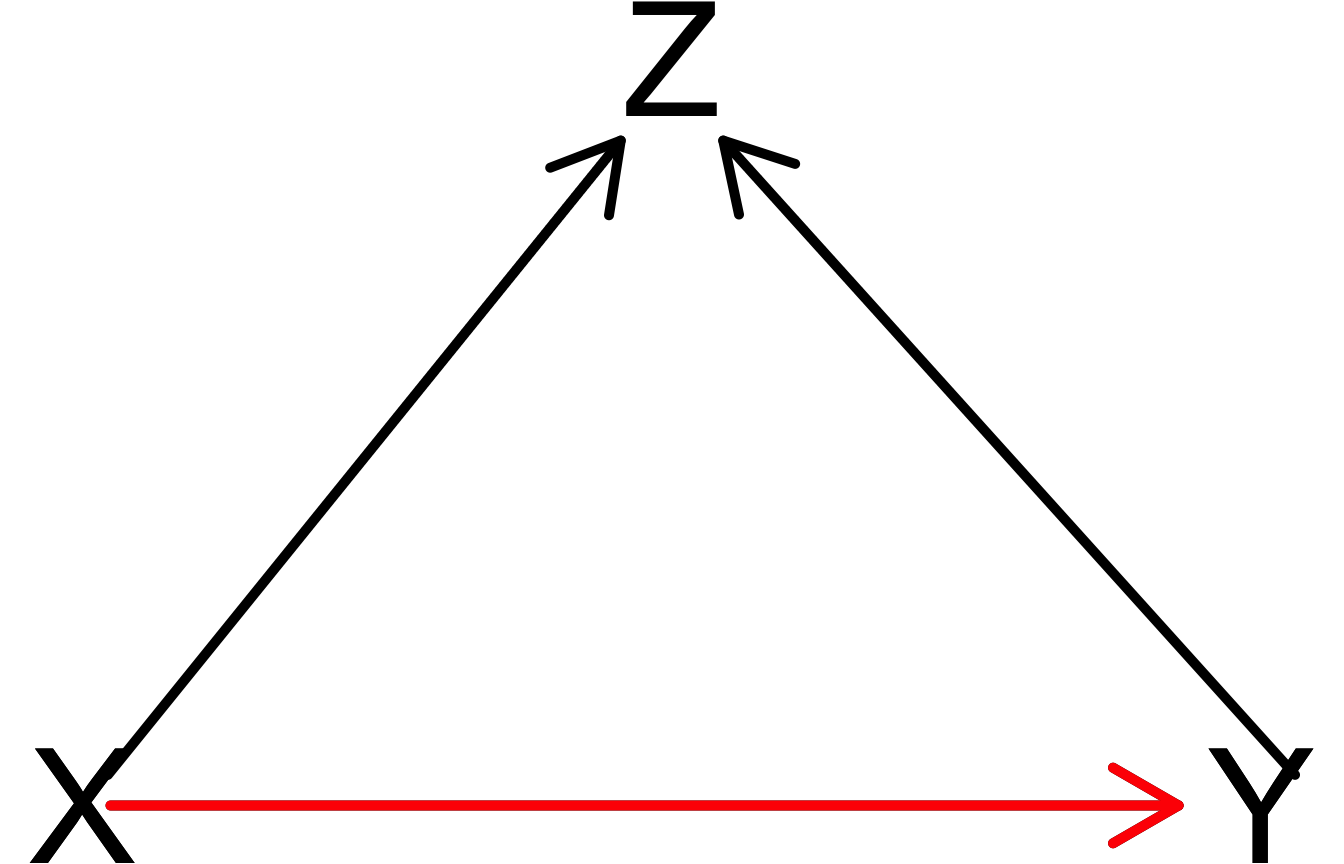
Forks \(X \leftarrow Z \rightarrow Y\): Conditioning = Blocking
Code
library(rethinking)
library(dagitty)
library(ggdag)
pipe_dag <-dagitty("dag{
X[exposure]
Y[outcome]
X -> Y
Z -> X
Z -> Y
}")
coordinates(pipe_dag) <- list(
    x=c(X=0, Z=0.5, Y=1),
    y=c(X=1, Z=0.5, Y=1)
)
drawdag_jj(pipe_dag, cex=5, lwd=5)
drawopenpaths_jj(pipe_dag, cex=5, lwd=5)
adj_sets <- adjustmentSets(
    pipe_dag, effect="direct"
)
writeLines("Adjustment sets (direct effect):")
adj_sets
library(ggtext)
set.seed(5650)
cfork_df <- tibble(
    Z = rbern(n_c),
    X = rnorm(n_c, 2 * Z - 1),
    Y = rnorm(n_c, 2 * Z - 1)
)
library(latex2exp)
overall_lm <- lm(Y ~ X, data=cfork_df)
overall_slope <- round(overall_lm$coef['X'], 3)
z0_lm <- lm(Y ~ X, data=cfork_df |> filter(Z == 0))
z0_slope <- round(z0_lm$coef['X'], 2)
z0_label <- paste0("<span style='color: #e69f00;'>Slope<sub>Z=0</sub> = ",z0_slope,"</span>")
z1_lm <- lm(Y ~ X, data=cfork_df |> filter(Z == 1))
z1_slope <- round(z1_lm$coef['X'], 2)
z1_label <- paste0("<span style='color: #56b4e9;'>Slope<sub>Z=1</sub> = ",z1_slope,"</span>")
z_texlabel <- paste0(z0_label, " | ", z1_label)
cfork_xmin <- min(cfork_df$X)
cfork_xmax <- max(cfork_df$X)
ggplot() +
  # Points
  geom_point(
    data=cfork_df,
    aes(x=X, y=Y, color=factor(Z)),
    size=0.4*g_pointsize,
    alpha=0.8
  ) +
  # Overall lm
  geom_smooth(
    data=cfork_df, aes(x=X, y=Y),
    method = lm, se = FALSE,
    linewidth = 2.75, color='white'
  ) +
  geom_smooth(
    data=cfork_df, aes(x=X, y=Y),
    method = lm, se = FALSE,
    linewidth = 2, color='black'
  ) +
  theme_dsan(base_size=18) +
  theme(
    plot.title = element_text(size=18),
    plot.subtitle = element_markdown(size=16)
  ) +
  # coord_equal() +
  labs(
    title = paste0(
      "Unstratified Slope = ",overall_slope
    ),
    x = "X", y = "Y", color = "Z"
  )

Adjustment sets (direct effect):
{ Z }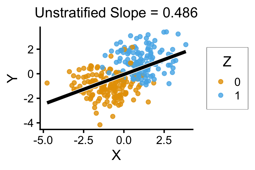
Code
fork_dag_closed <-dagitty("dag{
X[exposure]
Y[outcome]
Z[adjustedNode]
X -> Y
Z -> X
Z -> Y
}")
coordinates(fork_dag_closed) <- list(
    x=c(X=0, Z=0.5, Y=1),
    y=c(X=1, Z=0.5, Y=1)
)
fork_dag_closed <- setVariableStatus(
  fork_dag_closed, "adjustedNode", "Z"
)
drawdag_jj(
  fork_dag_closed, cex=5, lwd=5
)
drawopenpaths_jj(
  fork_dag_closed, Z="Z", lwd=5
)
library(ggtext)
set.seed(5650)
cfork_df <- tibble(
    Z = rbern(n_c),
    X = rnorm(n_c, 2 * Z - 1),
    Y = rnorm(n_c, 2 * Z - 1)
)
library(latex2exp)
overall_lm <- lm(Y ~ X, data=cfork_df)
overall_slope <- round(overall_lm$coef['X'], 3)
z0_lm <- lm(Y ~ X, data=cfork_df |> filter(Z == 0))
z0_slope <- round(z0_lm$coef['X'], 2)
z0_label <- paste0("<span style='color: #e69f00;'>Slope<sub>Z=0</sub> = ",z0_slope,"</span>")
z1_lm <- lm(Y ~ X, data=cfork_df |> filter(Z == 1))
z1_slope <- round(z1_lm$coef['X'], 2)
z1_label <- paste0("<span style='color: #56b4e9;'>Slope<sub>Z=1</sub> = ",z1_slope,"</span>")
z_texlabel <- paste0(z0_label, " | ", z1_label)
cfork_xmin <- min(cfork_df$X)
cfork_xmax <- max(cfork_df$X)
ggplot() +
  # Points
  geom_point(
    data=cfork_df,
    aes(x=X, y=Y, color=factor(Z)),
    size=0.4*g_pointsize,
    alpha=0.8
  ) +
  # Overall lm
  # geom_smooth(
  #   data=cfork_df, aes(x=X, y=Y),
  #   method = lm, se = FALSE,
  #   linewidth = 2.75, color='white'
  # ) +
  # geom_smooth(
  #   data=cfork_df, aes(x=X, y=Y),
  #   method = lm, se = FALSE,
  #   linewidth = 2, color='black'
  # ) +
  # Stratified lm
  # (slightly larger black lines)
  geom_smooth(
    data=cfork_df,
    aes(x=X, y=Y, group=factor(Z)),
    method=lm, se=FALSE, fullrange=TRUE,
    linewidth=2.75, color='black'
  ) +
  # (Colored lines)
  geom_smooth(
    data=cfork_df,
    aes(x=X, y=Y, color=factor(Z)),
    method=lm, se=FALSE, fullrange=TRUE,
    linewidth=2
  ) +
  theme_dsan(base_size=18) +
  theme(
    plot.title = element_text(size=18),
    plot.subtitle = element_markdown(size=16)
  ) +
  # coord_equal() +
  labs(
    # title = paste0(
    #   "Unstratified Slope = ",overall_slope
    # ),
    # subtitle=z_texlabel,
    subtitle=z_texlabel,
    x = "X", y = "Y", color = "Z"
  )

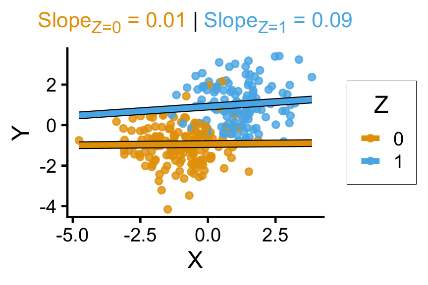
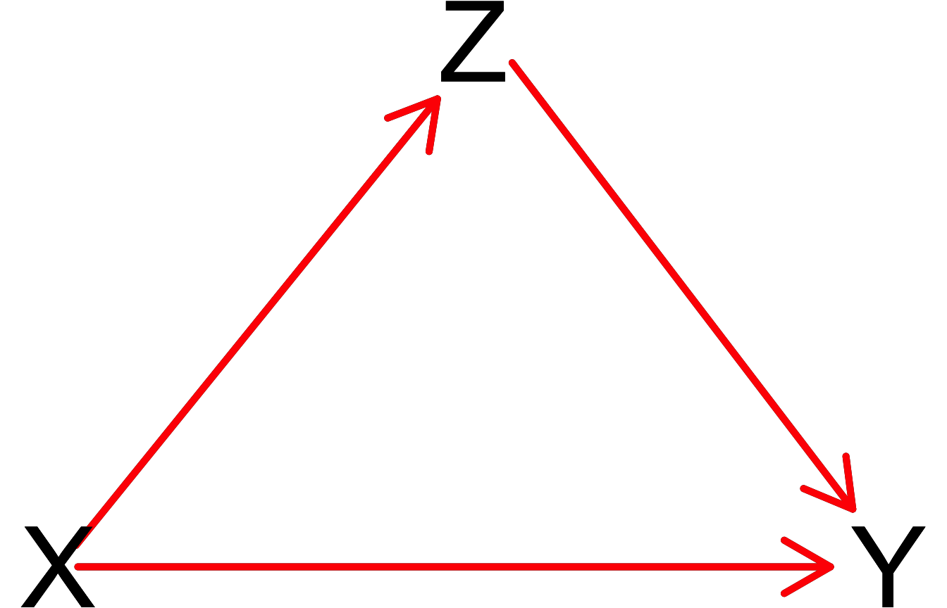
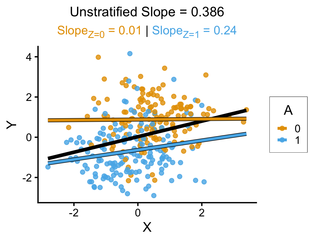
Conditioning on a Proxy for \(Z\)
- With just \(X \rightarrow Z \rightarrow Y\), we’d have a pipe
- Observing \(A \Rightarrow\) some (not all!) info about \(Z\)

Code
library(tidyverse)
library(extraDistr)
library(latex2exp)
set.seed(5650)
cprox_df <- tibble(
    X = rnorm(n_c),
    Z = rbern(n_c, plogis(X)),
    Y = rnorm(n_c, 2 * Z - 1),
    A = rbern(n_c, (1-Z)*0.86 + Z*0.14)
)
cprox_lm <- lm(Y ~ X, data=cprox_df)
cprox_slope <- round(cprox_lm$coef['X'], 3)
cprox_a0_lm <- lm(Y ~ X, data=cprox_df |> filter(A == 0))
cprox_a0_slope <- round(cprox_a0_lm$coef['X'], 2)
cprox_a0_label <- paste0("<span style='color: #e69f00;'>Slope<sub>Z=0</sub> = ",cprox_a0_slope,"</span>")
# A == 1 lm
cprox_a1_lm <- lm(Y ~ X, data=cprox_df |> filter(A == 1))
cprox_a1_slope <- round(cprox_a1_lm$coef['X'], 2)
cprox_a1_label <- paste0("<span style='color: #56b4e9;'>Slope<sub>Z=1</sub> = ",cprox_a1_slope,"</span>")
cprox_a_texlabel <- paste0(cprox_a0_label, " | ", cprox_a1_label)
cprox_xmin <- min(cprox_df$X)
cprox_xmax <- max(cprox_df$X)
ggplot() +
  # Points
  geom_point(
    data=cprox_df |> filter(Y > -3),
    aes(x=X, y=Y, color=factor(A)),
    size=0.5*g_pointsize,
    alpha=0.8
  ) +
  # Overall lm
  geom_smooth(
    data=cprox_df, aes(x=X, y=Y),
    method = lm, se = FALSE,
    linewidth = 2.5, color='black'
  ) +
  # Stratified lm
  # (slightly larger black lines)
  geom_smooth(
    data=cprox_df,
    aes(x=X, y=Y, group=factor(A)),
    method=lm, se=FALSE, fullrange=TRUE,
    linewidth=2.75, color='black'
  ) +
  # (Colored lines)
  geom_smooth(
    data=cprox_df,
    aes(x=X, y=Y, color=factor(A)),
    method=lm, se=FALSE, fullrange=TRUE,
    linewidth=2
  ) +
  theme_dsan(base_size=20) +
  theme(
    plot.title = element_text(size=20),
    plot.subtitle = element_markdown(size=18)
  ) +
  # coord_equal() +
  labs(
    title = paste0(
      "Unstratified Slope = ",cprox_slope
    ),
    subtitle=cprox_a_texlabel,
    x = "X", y = "Y", color = "A"
  )
⚠️Colliders⚠️ \(X \rightarrow Z \leftarrow Y\): Conditioning = Opening
Code
library(rethinking)
library(dagitty)
library(ggdag)
coll_dag <-dagitty("dag{
X[exposure]
Y[outcome]
X -> Y
X -> Z
Y -> Z
}")
coordinates(coll_dag) <- list(
    x=c(X=0, Z=0.5, Y=1),
    y=c(X=1, Z=0.5, Y=1)
)
drawdag_jj(
  coll_dag, cex=5, lwd=5
)
drawopenpaths_jj(coll_dag, lwd=5)
adj_sets_coll <- adjustmentSets(
    coll_dag, effect="direct"
)
writeLines("Adjustment sets (direct effect):")
adj_sets_coll
set.seed(5650)
ccoll_df <- tibble(
    X = rnorm(n_c),
    Y = rnorm(n_c),
    Z = rbern(n_c, plogis(2 * (X + Y - 1)))
)
ccoll_lm <- lm(Y ~ X, data=ccoll_df)
ccoll_slope <- round(ccoll_lm$coef['X'], 3)
ccoll_z0_lm <- lm(Y ~ X, data=ccoll_df |> filter(Z == 0))
ccoll_z0_slope <- round(ccoll_z0_lm$coef['X'], 2)
ccoll_z0_label <- paste0("<span style='color: #e69f00;'>Slope<sub>Z=0</sub> = ",ccoll_z0_slope,"</span>")
ccoll_z1_lm <- lm(Y ~ X, data=ccoll_df |> filter(Z == 1))
ccoll_z1_slope <- round(ccoll_z1_lm$coef['X'], 2)
ccoll_z1_label <- paste0("<span style='color: #56b4e9;'>Slope<sub>Z=1</sub> = ",ccoll_z1_slope,"</span>")
ccoll_z_texlabel <- paste0(ccoll_z0_label, " | ", ccoll_z1_label)
ccoll_xmin <- min(ccoll_df$X)
ccoll_xmax <- max(ccoll_df$X)
ggplot() +
  # Points
  geom_point(
    data=ccoll_df |> filter(Y > -3),
    aes(x=X, y=Y, color=factor(Z)),
    size=0.4*g_pointsize,
    alpha=0.8
  ) +
  # Overall lm
  geom_smooth(
    data=ccoll_df, aes(x=X, y=Y),
    method = lm, se = FALSE,
    linewidth = 2.75, color='white'
  ) +
  geom_smooth(
    data=ccoll_df, aes(x=X, y=Y),
    method = lm, se = FALSE,
    linewidth = 2, color='black'
  ) +
  theme_dsan(base_size=18) +
  theme(
    plot.title = element_markdown(size=18),
    plot.subtitle = element_markdown(size=16)
  ) +
  # coord_equal() +
  labs(
    # title=ccoll_z_texlabel,
    title=paste0("Unstratified Slope = ",ccoll_slope),
    x = "X", y = "Y", color = "Z"
  )

Adjustment sets (direct effect):
{}
Code
library(rethinking)
library(dagitty)
library(ggdag)
fork_dag_closed <- dagitty("dag{
X[exposure]
Y[outcome]
Z[adjustedNode]
X -> Y
X -> Z
Y -> Z
}")
coordinates(fork_dag_closed) <- list(
    x=c(X=0, Z=0.5, Y=1),
    y=c(X=1, Z=0.5, Y=1)
)
fork_dag_closed <- setVariableStatus(
  fork_dag_closed, "adjustedNode", "Z"
)
drawdag_jj(
  fork_dag_closed,
  cex=5, lwd=5,
)
drawopenpaths_jj(
  fork_dag_closed, Z="Z", lwd=5
)
set.seed(5650)
ccoll_df <- tibble(
    X = rnorm(n_c),
    Y = rnorm(n_c),
    Z = rbern(n_c, plogis(2 * (X + Y - 1)))
)
ccoll_lm <- lm(Y ~ X, data=ccoll_df)
ccoll_slope <- round(ccoll_lm$coef['X'], 3)
ccoll_z0_lm <- lm(Y ~ X, data=ccoll_df |> filter(Z == 0))
ccoll_z0_slope <- round(ccoll_z0_lm$coef['X'], 2)
ccoll_z0_label <- paste0("<span style='color: #e69f00;'>Slope<sub>Z=0</sub> = ",ccoll_z0_slope,"</span>")
ccoll_z1_lm <- lm(Y ~ X, data=ccoll_df |> filter(Z == 1))
ccoll_z1_slope <- round(ccoll_z1_lm$coef['X'], 2)
ccoll_z1_label <- paste0("<span style='color: #56b4e9;'>Slope<sub>Z=1</sub> = ",ccoll_z1_slope,"</span>")
ccoll_z_texlabel <- paste0(ccoll_z0_label, " | ", ccoll_z1_label)
ccoll_xmin <- min(ccoll_df$X)
ccoll_xmax <- max(ccoll_df$X)
ggplot() +
  # Points
  geom_point(
    data=ccoll_df |> filter(Y > -3),
    aes(x=X, y=Y, color=factor(Z)),
    size=0.4*g_pointsize,
    alpha=0.8
  ) +
  # Stratified lm
  # (slightly larger black lines)
  geom_smooth(
    data=ccoll_df,
    aes(x=X, y=Y, group=factor(Z)),
    method=lm, se=FALSE, fullrange=TRUE,
    linewidth=2.75, color='black'
  ) +
  # (Colored lines)
  geom_smooth(
    data=ccoll_df,
    aes(x=X, y=Y, color=factor(Z)),
    method=lm, se=FALSE, fullrange=TRUE,
    linewidth=2
  ) +
  theme_dsan(base_size=18) +
  theme(
    plot.title = element_markdown(size=18),
    plot.subtitle = element_markdown(size=16)
  ) +
  # coord_equal() +
  labs(
    title=ccoll_z_texlabel,
    x = "X", y = "Y", color = "Z"
  )


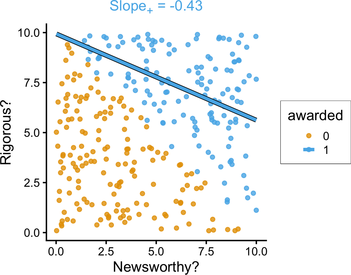
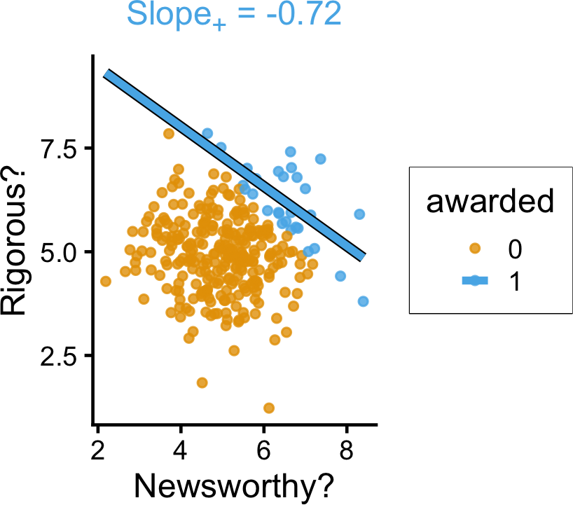
Is This Just a Corner Case?
- Grant applications are regularly judged on two criteria: novelty and rigor
- Judges grade proposal separately on the two criteria, grant is awarded to top \(N\) applications based on combined scores…
Code
set.seed(5650)
grant_df <- tibble(
    newsworthy = runif(n_c, 0, 10),
    rigorous = runif(n_c, 0, 10),
    awarded = ifelse(newsworthy + rigorous > 10, 1, 0)
)
grant_lm <- lm(rigorous ~ newsworthy, data=grant_df)
grant_slope <- round(grant_lm$coef['newsworthy'], 3)
grant_z0_lm <- lm(rigorous ~ newsworthy, data=grant_df |> filter(awarded == 0))
grant_z0_slope <- round(grant_z0_lm$coef['newsworthy'], 2)
grant_z1_lm <- lm(rigorous ~ newsworthy, data=grant_df |> filter(awarded == 1))
grant_z1_slope <- round(grant_z1_lm$coef['newsworthy'], 2)
grant_z1_label <- paste0("<span style='color: #56b4e9;'>Slope<sub>+</sub> = ",grant_z1_slope,"</span>")
grant_z_texlabel <- grant_z1_label
grant_xmin <- min(grant_df$newsworthy)
grant_xmax <- max(grant_df$newsworthy)
ggplot() +
  # Points
  geom_point(
    data=grant_df |> filter(rigorous > -3),
    aes(x=newsworthy, y=rigorous, color=factor(awarded)),
    size=0.4*g_pointsize,
    alpha=0.8
  ) +
  # Stratified lm
  # (slightly larger black lines)
  geom_smooth(
    data=grant_df |> filter(awarded == 1),
    aes(x=newsworthy, y=rigorous, group=factor(awarded)),
    method=lm, se=FALSE, fullrange=TRUE,
    linewidth=2.75, color='black'
  ) +
  # (Colored lines)
  geom_smooth(
    data=grant_df |> filter(awarded == 1),
    aes(x=newsworthy, y=rigorous, color=factor(awarded)),
    method=lm, se=FALSE, fullrange=TRUE,
    linewidth=2
  ) +
  theme_dsan(base_size=18) +
  theme(
    plot.title = element_markdown(size=18),
    plot.subtitle = element_markdown(size=16)
  ) +
  coord_equal() +
  labs(
    title=grant_z_texlabel,
    x = "Newsworthy?", y = "Rigorous?", color = "awarded"
  )
set.seed(5650)
grant_df <- tibble(
    newsworthy = rnorm(n_c, 5, 1),
    rigorous = rnorm(n_c, 5, 1),
    awarded = ifelse(newsworthy + rigorous > 12, 1, 0)
)
grant_lm <- lm(rigorous ~ newsworthy, data=grant_df)
grant_slope <- round(grant_lm$coef['newsworthy'], 3)
grant_z0_lm <- lm(rigorous ~ newsworthy, data=grant_df |> filter(awarded == 0))
grant_z0_slope <- round(grant_z0_lm$coef['newsworthy'], 2)
grant_z1_lm <- lm(rigorous ~ newsworthy, data=grant_df |> filter(awarded == 1))
grant_z1_slope <- round(grant_z1_lm$coef['newsworthy'], 2)
grant_z1_label <- paste0("<span style='color: #56b4e9;'>Slope<sub>+</sub> = ",grant_z1_slope,"</span>")
grant_z_texlabel <- grant_z1_label
grant_xmin <- min(grant_df$newsworthy)
grant_xmax <- max(grant_df$newsworthy)
ggplot() +
  # Points
  geom_point(
    data=grant_df |> filter(rigorous > -3),
    aes(x=newsworthy, y=rigorous, color=factor(awarded)),
    size=0.35*g_pointsize,
    alpha=0.8
  ) +
  # Stratified lm
  # (slightly larger black lines)
  geom_smooth(
    data=grant_df |> filter(awarded == 1),
    aes(x=newsworthy, y=rigorous, group=factor(awarded)),
    method=lm, se=FALSE, fullrange=TRUE,
    linewidth=2.75, color='black'
  ) +
  # (Colored lines)
  geom_smooth(
    data=grant_df |> filter(awarded == 1),
    aes(x=newsworthy, y=rigorous, color=factor(awarded)),
    method=lm, se=FALSE, fullrange=TRUE,
    linewidth=2
  ) +
  theme_dsan(base_size=18) +
  theme(
    plot.title = element_markdown(size=18),
    plot.subtitle = element_markdown(size=16)
  ) +
  coord_equal() +
  labs(
    title=grant_z_texlabel,
    x = "Newsworthy?", y = "Rigorous?", color = "awarded"
  )