Week 8: Propensity Score Weighting

DSAN 5650: Causal Inference for Computational Social Science
Summer 2025, Georgetown University

Jeff Jacobs

jj1088@georgetown.edu

Wednesday, July 9, 2025

Schedule

Today’s Planned Schedule:

	Start	End	Topic
Lecture	6:30pm	7:00pm	Final Project Pep Talk →
	7:00pm	7:50pm	Controlling For Things vs. Matching/Weighting →
Break!	7:50pm	8:00pm
	8:00pm	9:00pm	Propensity Score Lab →

\[ \DeclareMathOperator*{\argmax}{argmax} \DeclareMathOperator*{\argmin}{argmin} \newcommand{\bigexp}[1]{\exp\mkern-4mu\left[ #1 \right]} \newcommand{\bigexpect}[1]{\mathbb{E}\mkern-4mu \left[ #1 \right]} \newcommand{\definedas}{\overset{\small\text{def}}{=}} \newcommand{\definedalign}{\overset{\phantom{\text{defn}}}{=}} \newcommand{\eqeventual}{\overset{\text{eventually}}{=}} \newcommand{\Err}{\text{Err}} \newcommand{\expect}[1]{\mathbb{E}[#1]} \newcommand{\expectsq}[1]{\mathbb{E}^2[#1]} \newcommand{\fw}[1]{\texttt{#1}} \newcommand{\given}{\mid} \newcommand{\green}[1]{\color{green}{#1}} \newcommand{\heads}{\outcome{heads}} \newcommand{\iid}{\overset{\text{\small{iid}}}{\sim}} \newcommand{\lik}{\mathcal{L}} \newcommand{\loglik}{\ell} \DeclareMathOperator*{\maximize}{maximize} \DeclareMathOperator*{\minimize}{minimize} \newcommand{\mle}{\textsf{ML}} \newcommand{\nimplies}{\;\not\!\!\!\!\implies} \newcommand{\orange}[1]{\color{orange}{#1}} \newcommand{\outcome}[1]{\textsf{#1}} \newcommand{\param}[1]{{\color{purple} #1}} \newcommand{\pgsamplespace}{\{\green{1},\green{2},\green{3},\purp{4},\purp{5},\purp{6}\}} \newcommand{\pedge}[2]{\require{enclose}\enclose{circle}{~{#1}~} \rightarrow \; \enclose{circle}{\kern.01em {#2}~\kern.01em}} \newcommand{\pnode}[1]{\require{enclose}\enclose{circle}{\kern.1em {#1} \kern.1em}} \newcommand{\ponode}[1]{\require{enclose}\enclose{box}[background=lightgray]{{#1}}} \newcommand{\pnodesp}[1]{\require{enclose}\enclose{circle}{~{#1}~}} \newcommand{\purp}[1]{\color{purple}{#1}} \newcommand{\sign}{\text{Sign}} \newcommand{\spacecap}{\; \cap \;} \newcommand{\spacewedge}{\; \wedge \;} \newcommand{\tails}{\outcome{tails}} \newcommand{\Var}[1]{\text{Var}[#1]} \newcommand{\bigVar}[1]{\text{Var}\mkern-4mu \left[ #1 \right]} \]

library(tidyverse)
source("../dsan-globals/stat_binscatter.r")
source("../dsan-globals/_globals.r")

Roadmap for Part 2

• \(\downarrow\) Focus on abstract concepts / terminology
• \(\uparrow\) Focus on data analysis
• (Should hopefully start to feel more like other DSAN classes!)
• (\(\Rightarrow\) Need you to take specific examples I pick and analogize them to your field(s) of interest)

Final Projects

• Notion! Then, choose a path (rough draft of paths):
  • Modeling a social phenomenon with PGMs
  • Taking an existing project/interest (e.g., from 5300) and pushing towards the causality asymptote
• Choose a path by Tuesday, July 15, 6:30pm EDT

Propensity Score Weighting

• HW1 matching: similarity either 1 (applied to same schools) or 0 (didn’t apply to same schools)
• Propensity scores: model quality of match
• \(\Rightarrow\) Opens up (literally) infinite possibilities between 0 and 1!
• \(\Rightarrow\) Use your unsupervised learning skills (matching via clustering)
• \(\Rightarrow\) Use your supervised learning skills (propensity scores = logistic regression coefficients!)

Figure 1: Should this be matched with an apple? Or an orange? Porque no los dos! [Image source]

• \(\Rightarrow\) Use your diagnostic skills: e.g., methods for evaluating clusters / preventing overfitting

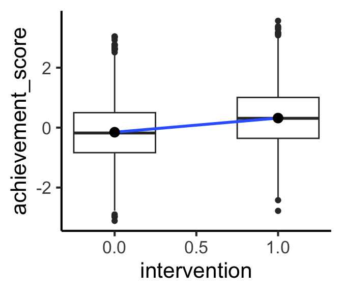
Working Example: Growth Mindset(!)

• From Athey and Wager (2019)
• Treatment \(T\), called intervention in the dataset: a seminar on growth mindset for high school students
• Outcome \(Y\), called achievement_score in the dataset: performance on state’s standardized test
• In a perfect world, we could just compute

\[ \mathbb{E}[Y \mid T = 1] - \mathbb{E}[Y \mid T = 0] \]

library(tidyverse)
library(broom)
student_df <- read_csv("assets/learning_mindset.csv")
(mean_df <- student_df |> group_by(intervention) |> summarize(mean_score=mean(achievement_score)))

intervention	mean_score
0	-0.1538030
1	0.3184686

student_naive_lm <- lm(achievement_score ~ intervention, data=student_df)
student_naive_lm |> broom::tidy() |> select(term, estimate)

term	estimate
(Intercept)	-0.1538030
intervention	0.4722717

student_df |>
  ggplot(aes(x=intervention, y=achievement_score)) +
  geom_boxplot(
    aes(group=intervention),
    width=0.5
  ) +
  geom_smooth(
    method='lm',
    formula='y ~ x',
    se=TRUE
  ) +
  geom_point(
    data=mean_df,
    aes(x=intervention, y=mean_score),
    size=3
  ) +
  theme_dsan(base_size=16)

The Problem: Pesky Covariates

• Here the “blob” \(\mathbf{X}\) forms a fork, as drawn…
• But in reality the work of modeling is flying into the cloud and modeling the \(\mathbf{X}\)-\(T\) and \(\mathbf{X}\)-\(Y\) relationships (especially: figuring out which covariates \(X_j \in \mathbf{X}\) are colliders), so you can close the backdoors:

• This can be really difficult, for a bunch of reasons… What if there was an easier way?

If We Had Control Over Everything (Experiments vs. Observational Data Analysis)

• If we could intervene in the DGP, we could assign treatment randomly, thus removing the impact of Covariates on \(T\)!

• Alas, we are data scientists, not (necessarily) experiment-conductors, plus there are often ethical reasons to not perform experiments!
• …There’s still another approach!

Closing Backdoors the Too-Good-To-Be-True Way

• Key insight from causal thinking: Transformation of the problem from “control for all covariates” to “close all backdoor paths”…
• For the goal of just closing these paths, we have an alternative¹:

• Rosenbaum and Rubin (1983): there exists a statistic \(\mathtt{e}(\mathbf{X}) = \Pr(T \mid \mathbf{X})\), the propensity score, which “captures” info in \(\textbf{X}\) relevant to \(T\) such that
• Conditioning on \(\mathtt{e}(\mathbf{X})\) closes \(\mathbf{X} \Rightarrow \mathtt{e}(\mathbf{X}) \rightarrow T\) (\(\mathtt{e}(\mathbf{X})\) is a pipe)

• This would close backdoor path \(T \leftarrow \mathtt{e}(\mathbf{X}) \Leftarrow \mathbf{X} \rightarrow Y\), leaving only direct effect \(T \rightarrow Y\)! There’s one remaining complication…

1. For reasons we’ll see later (double-robustness), you should ultimately try to achieve both goals!

Closing Backdoors via Propensity Score Estimation

• Sadly we don’t observe true probability of being treated for all possible values of \(\mathbf{X}\)
• But, we can derive an estimate \(\hat{\mathtt{e}}(\mathbf{X})\) using our machine learning skills 😎
• We now have that \(\hat{\mathtt{e}}(\mathbf{X})\), as a proxy relative to the pipe \(\mathbf{X} \Rightarrow \mathtt{e}(\mathbf{X}) \rightarrow T\), blocks the pipe to the extent that it captures the true probability \(\mathtt{e}(\mathbf{X}) = \Pr(T \mid \mathbf{X})\)

• Backdoor Path: \(T \leftarrow \mathtt{e}(\mathbf{X}) \Leftarrow \mathbf{X} \rightarrow Y\)
• Closed in proportion to \(\left[ \text{Cor}(\hat{\mathtt{e}}(\mathbf{X}), \mathtt{e}(\mathbf{X})) \right]^2 = ❓\)

Sometimes-Helpful Thought Experiment

• Back in our basic confounding scenario:
• If there was only one covariate (\(\mathbf{X} = X\)), and it was a constant (\(\Pr(X = c) = 1\)), then all the variation in \(Y\) would be due to variation in \(T\)
• Less extreme: if person \(i\) has covariates \(\mathbf{X}_i\) and person \(j\) has covariates \(\mathbf{X}_j\), but \(\mathbf{X}_i = \mathbf{X}_j\), then variation in their outcomes is due solely to \(T\)

• Part of the logic of propensity score is that, if person \(i\) has covariates \(\mathbf{X}_i\) and person \(j\) has covariates \(\mathbf{X}_j\), but \(\mathtt{e}(\mathbf{X}_i) = \mathtt{e}(\mathbf{X}_j)\), then \(i\) and \(j\) are perfectly matched
• \(\Rightarrow\) (by fun math proof) variation in their outcomes is due solely to \(T\)

How Exactly Do We Adjust For \(\hat{\mathtt{e}}(\mathbf{X})\)?

• Simulation example: smoking reduction

library(tidyverse)
library(Rlab)
set.seed(5650)
n <- 250
motiv_vals <- runif(n, 0, 1)
enroll_vals <- ifelse(
  motiv_vals < 0.25,
  0,
  # We know motiv > 0.25
  ifelse(
    motiv_vals > 0.75,
    1,
    # We know 0.25 < motiv < 0.75
    rbern(n, prob=(motiv_vals - 0.125)*1.5)
  )
)
ncigs_vals <- rbinom(n, size=30, prob=0.6-0.2*enroll_vals)
smoke_df <- tibble(
  motiv=motiv_vals,
  enroll=enroll_vals,
  ncigs=ncigs_vals
)
(smoke_mean_df <- smoke_df |> group_by(enroll) |> summarize(mean_ncigs=mean(ncigs)))

enroll	mean_ncigs
0	17.88060
1	12.26724

naive_smoke_lm <- lm(ncigs ~ enroll, data=smoke_df)
summary(naive_smoke_lm) |> broom::tidy() |>
  select(term, estimate)

term	estimate
(Intercept)	17.880597
enroll	-5.613356

smoke_df |> ggplot(aes(x=enroll, y=ncigs)) +
  geom_boxplot(
    aes(group=enroll),
    width=0.5
  ) +
  geom_smooth(
    method='lm',
    formula='y ~ x',
    se=TRUE
  ) +
  geom_point(
    data=smoke_mean_df,
    aes(x=enroll, y=mean_ncigs),
    size=3
  ) +
  theme_dsan(base_size=24)

Inverse Probability-of-Treatment Weighting

eprop_model <- glm(enroll ~ motiv, family='binomial', data=smoke_df)
eprop_preds <- predict(eprop_model, type="response")
smoke_df <- smoke_df |> mutate(pred=eprop_preds)
# Use the preds to compute IPW
smoke_df <- smoke_df |> rowwise() |> mutate(
  ipw=ifelse(enroll, 1/pred, 1/(1-pred))
) |> arrange(pred)
#smoke_df
smoke_df |> mutate(enroll=factor(enroll)) |>
  ggplot(aes(x=motiv, y=ncigs, color=enroll)) +
  geom_point() +
  theme_dsan(base_size=24) +
  labs(title="Before Weighting")

smoke_df |> mutate(enroll=factor(enroll)) |>
  ggplot(aes(
    x=motiv, y=ncigs, color=enroll, size=ipw,
    alpha=log(ipw-1)
  )) +
  geom_point() +
  guides(alpha="none") +
  theme_dsan(base_size=24) +
  labs(title="After Weighting")

smoke_df |>
  ggplot(aes(x=motiv)) +
  # Predictions
  geom_point(
    aes(y=enroll, color=factor(enroll))
  ) +
  # Values
  geom_point(
    aes(y=pred, color=factor(enroll))
  ) +
  labs(color="enroll") +
  theme_dsan(base_size=24) +
  labs(title="Propensity to Enroll")
ipw_min <- min(smoke_df$ipw)
ipw_max <- max(smoke_df$ipw)
smoke_df <- smoke_df |> mutate(
  ipw_scaled = (ipw - ipw_min) / (ipw_max - ipw_min)
)
smoke_df |>
  ggplot(aes(x=motiv)) +
  # Predictions
  geom_point(
    aes(y=enroll, color=factor(enroll))
  ) +
  # Values
  geom_point(
    aes(y=ipw_scaled, color=factor(enroll))
  ) +
  theme_dsan(base_size=24) +
  labs(
    title="Inverse Probability-of-Treatment Weights (IPTW)",
    color="enroll"
  )

↓

→

↑

The Final Result!

lm_with_weights <- lm(ncigs ~ enroll,
  data=smoke_df, weights=smoke_df$ipw
)
summary(lm_with_weights) |> broom::tidy() |>
  select(term, estimate, std.error)

term	estimate	std.error
(Intercept)	18.10133	0.2466712
enroll	-5.66453	0.3571696

library(WeightIt)
W <- weightit(
  enroll ~ motiv, data = smoke_df, ps="pred"
)
smoke_weighted_lm <- lm_weightit(
  ncigs ~ enroll, data = smoke_df, weightit = W
)
summary(smoke_weighted_lm, ci = FALSE)

Call:
lm_weightit(formula = ncigs ~ enroll, data = smoke_df, weightit = W)

Coefficients:
            Estimate Std. Error z value Pr(>|z|)    
(Intercept)  18.1013     0.2479   73.02   <1e-06 ***
enroll       -5.6645     0.5463  -10.37   <1e-06 ***
Standard error: HC0 robust

W_default <- weightit(enroll ~ motiv, data = smoke_df)
smoke_default_lm <- lm_weightit(
  ncigs ~ enroll, data = smoke_df,
  weightit = W_default
)
summary(smoke_default_lm, ci = FALSE)

Call:
lm_weightit(formula = ncigs ~ enroll, data = smoke_df, weightit = W_default)

Coefficients:
            Estimate Std. Error z value Pr(>|z|)    
(Intercept)  18.1013     0.2441   74.16   <1e-06 ***
enroll       -5.6645     0.5444  -10.41   <1e-06 ***
Standard error: HC0 robust (adjusted for estimation of weights)

…What If We Have Many Covariates?

• Curse of dimensionality…
• Lab Time!

References

Athey, Susan, and Stefan Wager. 2019. “Estimating Treatment Effects with Causal Forests: An Application.” arXiv. https://doi.org/10.48550/arXiv.1902.07409.

Rosenbaum, Paul R., and Donald B. Rubin. 1983. “The Central Role of the Propensity Score in Observational Studies for Causal Effects.” Biometrika 70 (1): 41–55. https://doi.org/10.2307/2335942.