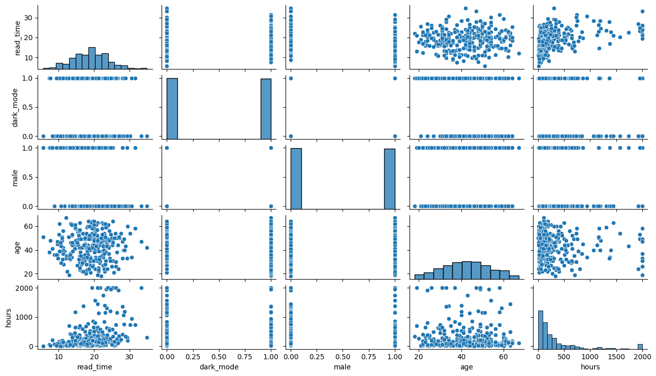
| read_time | dark_mode | male | age | hours | |
|---|---|---|---|---|---|
| 0 | 14.4 | False | 0 | 43.0 | 65.6 |
| 1 | 15.4 | False | 1 | 55.0 | 125.4 |
| 2 | 20.9 | True | 0 | 23.0 | 642.6 |
| 3 | 20.0 | False | 0 | 41.0 | 129.1 |
| 4 | 21.5 | True | 0 | 29.0 | 190.2 |
DSAN 5650: Causal Inference for Computational Social Science
Summer 2026, Georgetown University
Wednesday, July 22, 2026
Today’s Planned Schedule:
| Start | End | Topic | |
|---|---|---|---|
| Lecture | 6:30pm | 6:45pm | Final Projects → |
| 6:45pm | 7:10pm | Instrumental Variables Lite → | |
| 7:30pm | 8:00pm | When Conditioning Won’t Cut It: IVs → | |
| 7:10pm | 8:00pm | Text-as-Data Part 1: TAD in General → | |
| Break! | 8:00pm | 8:10pm | |
| 8:10pm | 9:00pm | Text-as-Data Part 2: Causal Text Analysis → |
\[ \DeclareMathOperator*{\argmax}{argmax} \DeclareMathOperator*{\argmin}{argmin} \newcommand{\bigexp}[1]{\exp\mkern-4mu\left[ #1 \right]} \newcommand{\bigexpect}[1]{\mathbb{E}\mkern-4mu \left[ #1 \right]} \newcommand{\definedas}{\overset{\small\text{def}}{=}} \newcommand{\definedalign}{\overset{\phantom{\text{defn}}}{=}} \newcommand{\eqeventual}{\overset{\text{eventually}}{=}} \newcommand{\Err}{\text{Err}} \newcommand{\expect}[1]{\mathbb{E}[#1]} \newcommand{\expectsq}[1]{\mathbb{E}^2[#1]} \newcommand{\fw}[1]{\texttt{#1}} \newcommand{\given}{\mid} \newcommand{\green}[1]{\color{green}{#1}} \newcommand{\heads}{\outcome{heads}} \newcommand{\iid}{\overset{\text{\small{iid}}}{\sim}} \newcommand{\lik}{\mathcal{L}} \newcommand{\loglik}{\ell} \DeclareMathOperator*{\maximize}{maximize} \DeclareMathOperator*{\minimize}{minimize} \newcommand{\mle}{\textsf{ML}} \newcommand{\nimplies}{\;\not\!\!\!\!\implies} \newcommand{\orange}[1]{\color{orange}{#1}} \newcommand{\outcome}[1]{\textsf{#1}} \newcommand{\param}[1]{{\color{purple} #1}} \newcommand{\pgsamplespace}{\{\green{1},\green{2},\green{3},\purp{4},\purp{5},\purp{6}\}} \newcommand{\pedge}[2]{\require{enclose}\enclose{circle}{~{#1}~} \rightarrow \; \enclose{circle}{\kern.01em {#2}~\kern.01em}} \newcommand{\pnode}[1]{\require{enclose}\enclose{circle}{\kern.1em {#1} \kern.1em}} \newcommand{\ponode}[1]{\require{enclose}\enclose{box}[background=lightgray]{{#1}}} \newcommand{\pnodesp}[1]{\require{enclose}\enclose{circle}{~{#1}~}} \newcommand{\purp}[1]{\color{purple}{#1}} \newcommand{\sign}{\text{Sign}} \newcommand{\spacecap}{\; \cap \;} \newcommand{\spacewedge}{\; \wedge \;} \newcommand{\tails}{\outcome{tails}} \newcommand{\Var}[1]{\text{Var}[#1]} \newcommand{\bigVar}[1]{\text{Var}\mkern-4mu \left[ #1 \right]} \]
🥳 You’re doing great 🥳
With doubly-robust estimation, as long as the answer is either True or False you’re good!

import pandas as pd
import numpy as np
import matplotlib.pyplot as plt
import seaborn as sns
from IPython.display import HTML
import statsmodels.formula.api as smf
from causalml.match import create_table_one
from joblib import Parallel, delayed
from sklearn.linear_model import LogisticRegression
def generate_data(N=300, seed=1):
np.random.seed(seed)
# Control variables
male = np.random.binomial(1, 0.45, N)
age = np.rint(18 + np.random.beta(2, 2, N)*50)
hours = np.minimum(np.round(np.random.lognormal(5, 1.3, N), 1), 2000)
# Treatment
pr = np.maximum(0, np.minimum(1, 0.8 + 0.3*male - np.sqrt(age-18)/10))
dark_mode = np.random.binomial(1, pr, N)==1
# Outcome
read_time = np.round(np.random.normal(10 - 4*male + 2*np.log(hours) + 2*dark_mode, 4, N), 1)
# Generate the dataframe
df = pd.DataFrame({'read_time': read_time, 'dark_mode': dark_mode, 'male': male, 'age': age, 'hours': hours})
return df
user_df = generate_data(N=300)
ols_model = smf.ols("read_time ~ dark_mode", data=user_df).fit()
ols_summary = ols_model.summary()
results_as_html = ols_summary.tables[1].as_html()
HTML(results_as_html)| coef | std err | t | P>|t| | [0.025 | 0.975] | |
|---|---|---|---|---|---|---|
| Intercept | 19.1748 | 0.402 | 47.661 | 0.000 | 18.383 | 19.967 |
| dark_mode[T.True] | -0.4446 | 0.571 | -0.779 | 0.437 | -1.568 | 0.679 |
…So, is this a causal effect? Does dark theme cause users to spend less time reading?
(…since I couldn’t figure out how to fit it on the last slide)
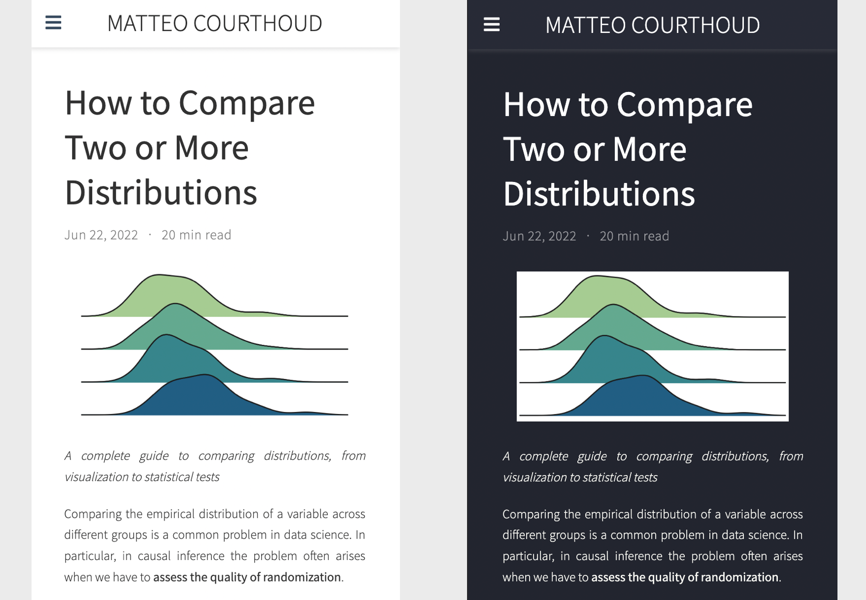
Enter Uber’s causal inference library: causalml
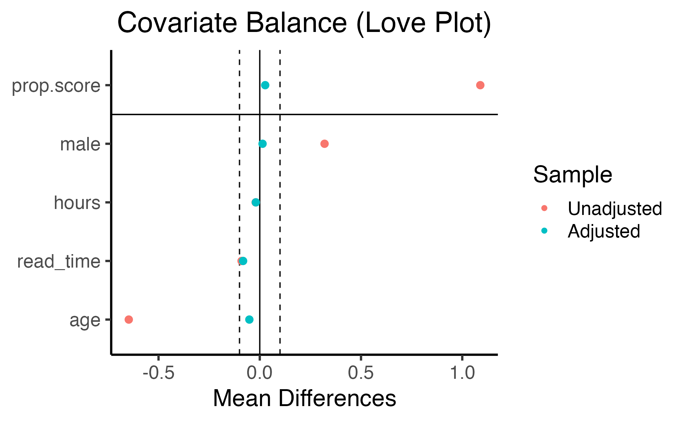
| Control | Treatment | SMD | |
|---|---|---|---|
| Variable | |||
| n | 151 | 149 | |
| age | 46.01 (9.79) | 39.09 (11.53) | -0.6469 |
| hours | 337.78 (464.00) | 328.57 (442.12) | -0.0203 |
| male | 0.34 (0.47) | 0.66 (0.48) | 0.6732 |
And then WeightIt to generate a “love plot”:
\[ \hat\tau = \frac{1}{n}\sum_i \left[ \hat\mu_1(X_i) - \hat\mu_0(X_i) + \frac{T_i(Y_i - \hat\mu_1(X_i))}{\hat e(X_i)} - \frac{(1-T_i)(Y_i - \hat\mu_0(X_i))}{1-\hat e(X_i)} \right] \]
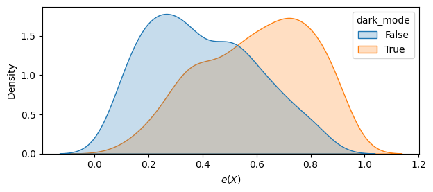
def estimate_e(df, X, D, model_e):
e = model_e.fit(df[X], df[D]).predict_proba(df[X])[:,1]
return e
user_df['e'] = estimate_e(user_df, X, "dark_mode", LogisticRegression())
fig, ax = plt.subplots(figsize=(7,2.75))
sns.kdeplot(
x='e', hue='dark_mode', data=user_df,
# bins=30,
#stat='density',
common_norm=False,
fill=True,
ax=ax
);
ax.set_xlabel("$e(X)$");
| coef | std err | t | P>|t| | [0.025 | 0.975] | |
|---|---|---|---|---|---|---|
| Intercept | 18.5871 | 0.412 | 45.158 | 0.000 | 17.777 | 19.397 |
| dark_mode[T.True] | 1.0486 | 0.581 | 1.805 | 0.072 | -0.095 | 2.192 |
First, with scikit-learn:
from sklearn.linear_model import LinearRegression
def estimate_mu(df, X, D, y, model_mu):
mu = model_mu.fit(df[X + [D]], df[y])
mu0 = mu.predict(df[X + [D]].assign(dark_mode=0))
mu1 = mu.predict(df[X + [D]].assign(dark_mode=1))
return mu0, mu1
mu0, mu1 = estimate_mu(
user_df, X, "dark_mode", "read_time", LinearRegression()
)
print(f'mean(mu0) = {np.mean(mu0):.2f}, mean(mu1) = {np.mean(mu1):.2f}')
print(f'Difference = {np.mean(mu1 - mu0):.2f}')mean(mu0) = 18.27, mean(mu1) = 19.65
Difference = 1.39
Enter EconML, Microsoft’s “Official” ML-based econometrics library 😎
from econml.dr import LinearDRLearner
model = LinearDRLearner(
model_propensity=LogisticRegression(),
model_regression=LinearRegression(),
random_state=5650
)
model.fit(Y=user_df["read_time"], T=user_df["dark_mode"], X=user_df[X]);
model.ate_inference(X=user_df[X].values, T0=0, T1=1).summary().tables[0]| mean_point | stderr_mean | zstat | pvalue | ci_mean_lower | ci_mean_upper |
|---|---|---|---|---|---|
| 1.321 | 0.549 | 2.409 | 0.016 | 0.246 | 2.396 |
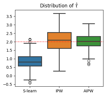
Wrong regression model:
def compare_estimators(X_e, X_mu, D, y, seed):
df = generate_data(seed=seed)
e = estimate_e(df, X_e, D, LogisticRegression())
mu0, mu1 = estimate_mu(df, X_mu, D, y, LinearRegression())
slearn = mu1 - mu0
ipw = (df[D] / e - (1-df[D]) / (1-e)) * df[y]
aipw = slearn + df[D] / e * (df[y] - mu1) - (1-df[D]) / (1-e) * (df[y] - mu0)
return np.mean((slearn, ipw, aipw), axis=1)
def simulate_estimators(X_e, X_mu, D, y):
r = Parallel(n_jobs=8)(delayed(compare_estimators)(X_e, X_mu, D, y, i) for i in range(100))
df_tau = pd.DataFrame(r, columns=['S-learn', 'IPW', 'AIPW'])
return df_tau
# The actual plots
fig, ax = plt.subplots(figsize=(4,3.5))
wrong_reg_df = simulate_estimators(
X_e=['male', 'age'], X_mu=['hours'], D="dark_mode", y="read_time"
)
wrong_reg_plot = sns.boxplot(
data=pd.melt(wrong_reg_df), x='variable', y='value', hue='variable',
ax=ax,
linewidth=2
);
wrong_reg_plot.set(
title="Distribution of $\hat τ$", xlabel='', ylabel=''
);
ax.axhline(2, c='r', ls=':');
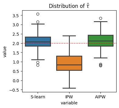
Wrong propensity score model:
fig, ax = plt.subplots(figsize=(4, 3.5))
wrong_ps_df = simulate_estimators(
['age'], ['male', 'hours'], D="dark_mode", y="read_time"
)
wrong_ps_plot = sns.boxplot(
data=pd.melt(wrong_ps_df), x='variable', y='value', hue='variable',
ax=ax,
linewidth=2
);
ax.set_title("Distribution of $\hat τ$");
ax.axhline(2, c='r', ls=':');
plt.show()
If randomization works to obtain causal effects…
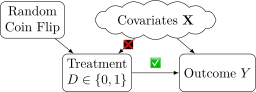
…Find something random in the causal system, use e.g. matching to “force” the same scenario!
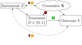
General form: \(\text{Effect}(D \rightarrow Y) = \frac{\text{Effect}(Z \rightarrow Y)}{\text{Effect}(Z \rightarrow D)}\) (Try “plugging in” \(Z\) = Coin Flip!)
\[ \beta_{\text{IV}}^{\text{Wald}} = \frac{ \mathbb{E}[Y_i \mid Z_i = 1] - \mathbb{E}[Y_i \mid Z_i = 0] }{ \mathbb{E}[D_i \mid Z_i = 1] - \mathbb{E}[D_i \mid Z_i = 0] }, \; \beta_{\text{IV}} = \frac{\text{Cov}[Y, Z]}{\text{Cov}[D,Z]} \]
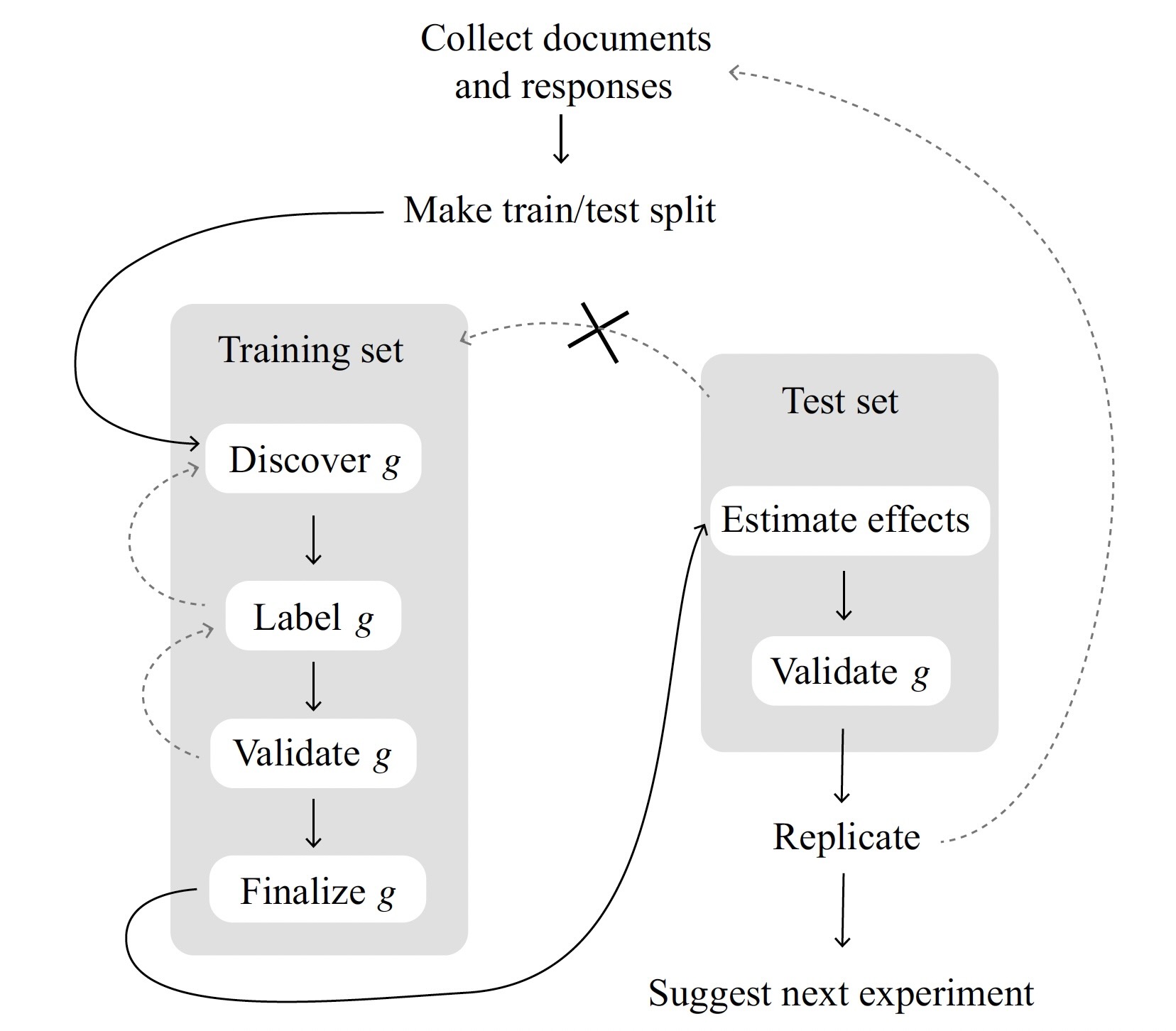
(The necessity for sample splitting!)
| \(Y_i \mid \textsf{do}(D_i \leftarrow 1)\) | \(Y_i \mid \textsf{do}(D_i \leftarrow 0)\) | |
|---|---|---|
| Person 1 | Candidate’s Morals | Taxes |
| Person 2 | Candidate’s Morals | Taxes |
| Person 3 | Polarization | Immigration |
| Person 4 | Polarization | Immigration |
| \(Y_i \mid \textsf{do}(D_i \leftarrow 1)\) | \(Y_i \mid \textsf{do}(D_i \leftarrow 0)\) | |
|---|---|---|
| Person 1 | Candidate’s Morals | Taxes |
| Person 2 | Candidate’s Morals | Taxes |
| Person 3 | Polarization | Immigration |
| Person 4 | Polarization | Immigration |
| Actual Assignment | Outcome \(Y_i\) | |
|---|---|---|
| Person 1 | \(D_1 = 1\) | Morals |
| Person 2 | \(D_2 = 1\) | Morals |
| Person 3 | \(D_3 = 0\) | Immigration |
| Person 4 | \(D_4 = 0\) | Immigration |
| Actual Assignment | Outcome \(Y_i\) | |
|---|---|---|
| Person 1 | \(D_1 = 1\) | Morals |
| Person 2 | \(D_2 = 0\) | Taxes |
| Person 3 | \(D_3 = 1\) | Polarization |
| Person 4 | \(D_4 = 0\) | Immigration |
| Section | Keywords |
|---|---|
| U.S. News | state, court, federal, republican |
| World News | government, country, officials, minister |
| Arts | music, show, art, dance |
| Sports | game, league, team, coach |
| Real Estate | home, bedrooms, bathrooms, building |
| Arts | Real Estate | Sports | U.S. News | World News | |
|---|---|---|---|---|---|
| Correct | 3020 | 690 | 4860 | 1330 | 1730 |
| Incorrect | 750 | 60 | 370 | 1100 | 590 |
| Accuracy | 0.801 | 0.920 | 0.929 | 0.547 | 0.746 |
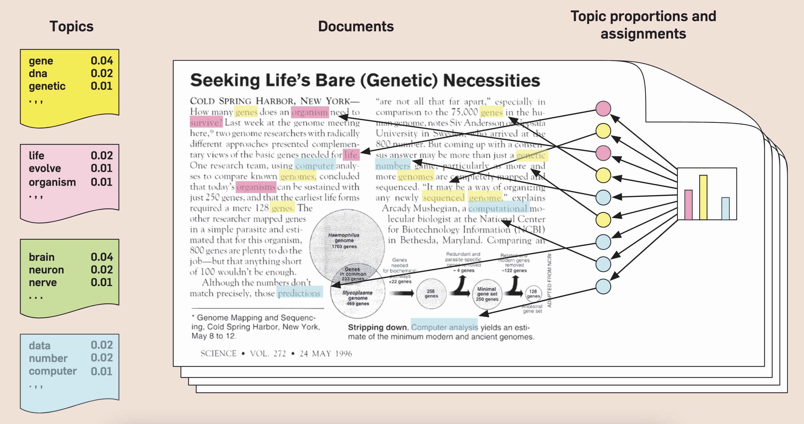
From Blei (2012)
…Unlocks a world of social modeling through text!
Blaydes et al. (2018)
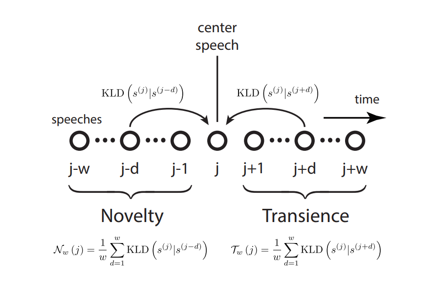
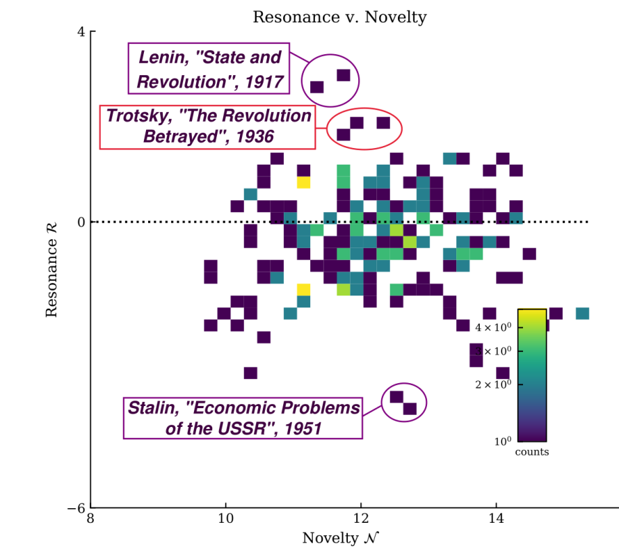
From Barron et al. (2018)
DSAN 5650 Week 10: Text-as-Data