source("../dsan-globals/_globals.r")Week 13: SWFLs, Identity Formation, and Discourse Ethics
DSAN 5450: Data Ethics and Policy
Spring 2026, Georgetown University
Class Sessions
Last Week: Social Welfare Functionals
(Fun notation:)
- SWF \(w(x)\) = Social Welfare Function:
- Plug in a Policy \(x\), obtain a Welfare “Level” \(y \in \mathbb{R}\)
- Policy \(x_1\) “better than” policy \(x_0\) iff \(w(x_1) > w(x_0)\)
- But how do we construct this function? Two antecedents:
- Methodological individualism: groups don’t have “preferences” as such; individuals do (if you ask a group for their opinion, how is answer generated? Discussion? Voting? Dictatorship?)
- Ideal speech situation: Habermas (1990) (later/next week)
- SWFL \(W(\mathbf{u})\) = Social Welfare Functional (Sen 1970): Explicit account of “social preference” as aggregation of individual preferences!
- Plug in Utility profile \((u_1(\cdot), \ldots, u_n(\cdot))\), obtain SWF \(w(x)\)
- \(W(\mathbf{u})(x)\) = Aggregate individual preferences via \(W(\mathbf{u})\) (producing a SWF), then evaluate this aggregation at \(x\)


Functionals?
- You probably know what a function \(f(x)\) is; a functional is a function of functions: \(\mathscr{G}(f)\)
- Letters get bigger/curlier, which is scary, but the notation is there to remind us that we need to consider two steps: What are the “base level” functions \(f\), and how are they aggregated?
- For our purposes, they “work the same” as regular functions
- Ex: If \(\mathscr{G}(f,g) = f^2 + g^2, f(x) = x, g(x) = 2x\), then we can obtain \(\mathscr{G}(f,g)(x)\) by evaluating \(f(x)\), \(g(x)\), and combining:
\[ \mathscr{G}(f,g)(2) = (\underbrace{2}_{\mathclap{f(2)}})^2 + (\underbrace{2(2)}_{\mathclap{g(2)}})^2 = 20 \]
We Live In A Dang Society
- Utilitarianism, Kant, Rawls can all be modeled as Social Welfare Functionals
\[ W(\mathbf{u}) = W(u_1, \ldots, u_n) \Rightarrow W(\mathbf{u})(x) = W(u_1(x), \ldots, u_n(x)) \]
- \(u_i(x)\): Given bundle of resources \(x\), how much utility does \(i\) experience? \(u_i: \mathcal{X} \rightarrow \mathbb{R}\)
- \(W(\mathbf{u})\): Aggregates \(u_i(x)\) over all \(i\), to produce measure of overall welfare of society. For \(N\) people, \(W: (\underbrace{\mathcal{X} \rightarrow \mathbb{R}}_{u_i(\cdot)})^N \rightarrow \mathbb{R}\).
- Standard assumption: \(W\) additive \(\Rightarrow W(\mathbf{u}) = \sum_{i=1}^n \omega_iu_i(x)\)
- \(\omega_i \equiv \frac{\partial W}{\partial u_i}\) is \(i\)’s welfare weight (❗️)
- Welfare-Economic definition of Utilitarianism: Literally just \(\omega_i = \frac{1}{n} \; \forall i\)
- (HW4) Decomposition to evaluate bias in policy impacts: from observed allocation \(x_i\) and marginal utility \(u'_i(x)\), can…
- Infer \(\widehat{\omega}_i\) (how much policy does value person \(i\): descriptive), then
- Compare with \(\omega_i^*\) (how much policy should value person \(i\): normative 🤯)
Alternative SWF Specifications
- Social values
\[ W(\underbrace{v_1, \ldots, v_n}_{\text{Values}})(x) \overset{\text{e.g.}}{=} \omega_1\underbrace{v_1(x)}_{\text{Privacy}} + \omega_2\underbrace{v_2(x)}_{\mathclap{\text{Public Health}}} \]
- Stakeholder Analysis
\[ W(\underbrace{s_1, \ldots, s_n}_{\text{Stakeholders}})(x) = \omega_1\underbrace{u_{s_1}(x)}_{\text{Teachers}} + \omega_2\underbrace{u_{s_2}(x)}_{\text{Parents}} + \omega_3\underbrace{u_{s_3}(x)}_{\text{Students}} + \omega_4\underbrace{u_{s_4}(x)}_{\mathclap{\text{Community}}} \]
- (Adapted from this great intro video!)
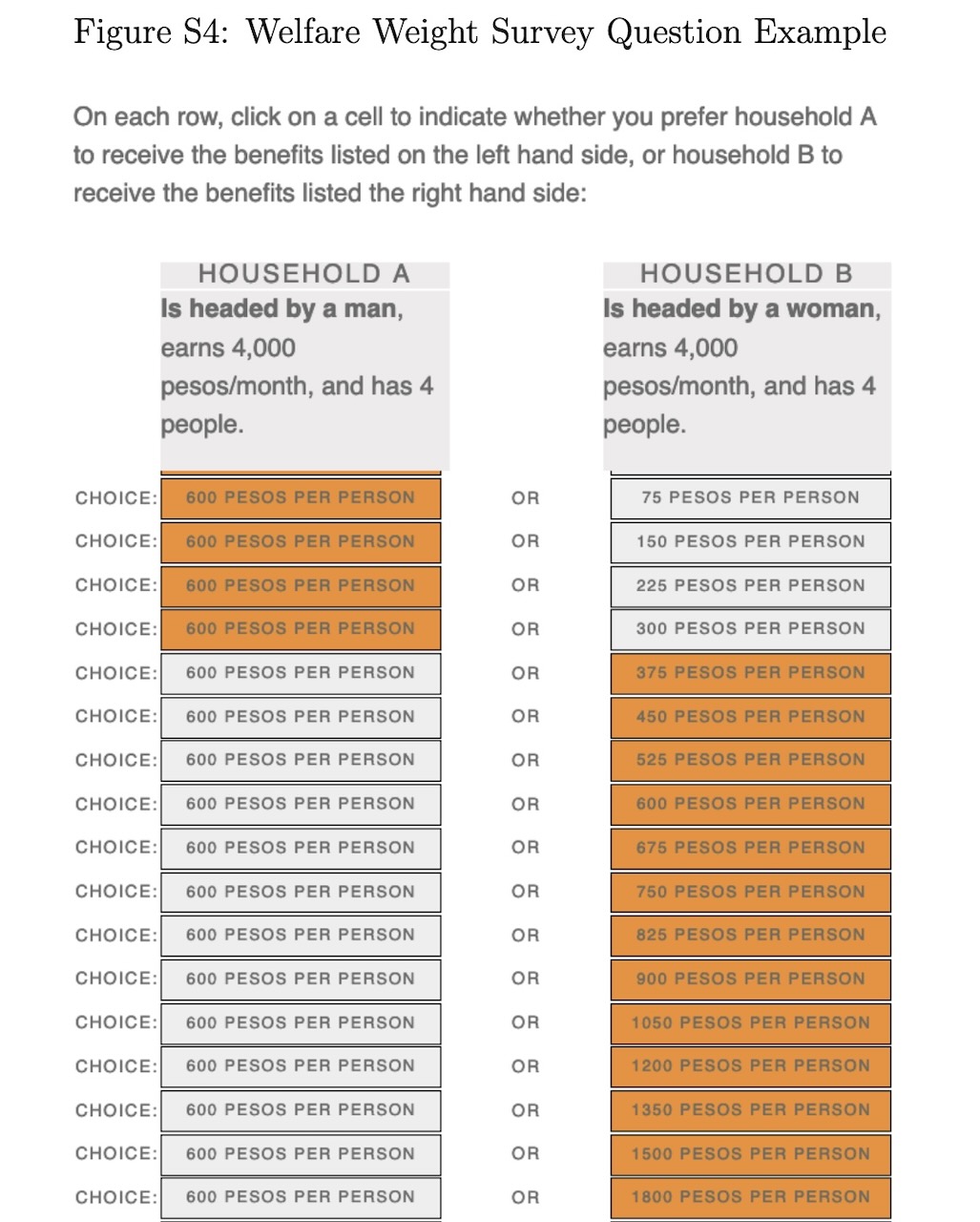
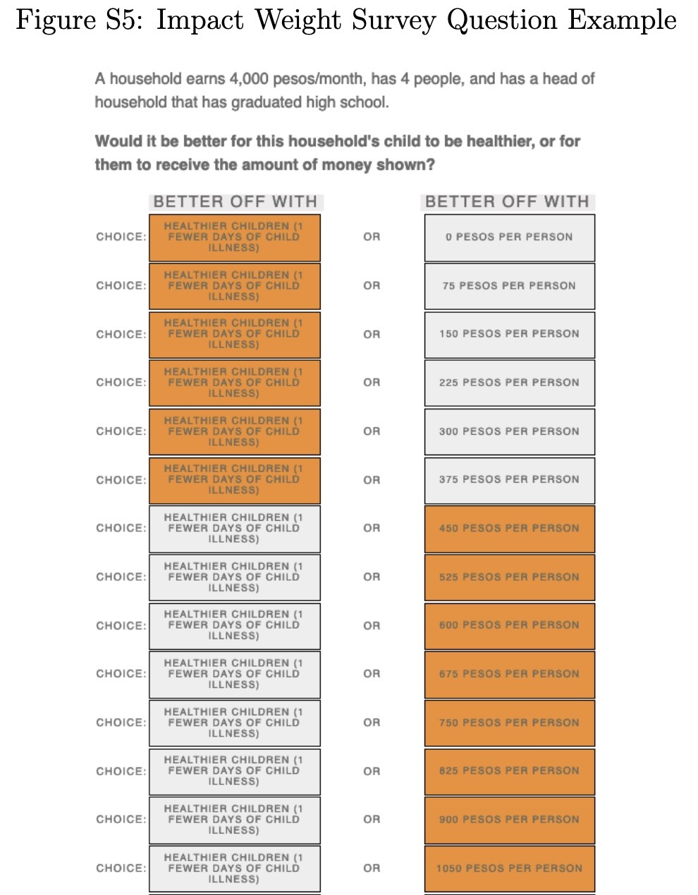
Inferring SWF from Surveys
“Conjoint Study”!
The Conveniently-Left-Out Detail
- Recall, e.g., predictive parity:
\[ \mathbb{E}[Y \mid D = 1, A = 1] = \mathbb{E}[Y \mid D = 1, A = 0] \]
- Who decides which \(Y\) to pick? (Kasy and Abebe 2021)
- Answer: Whoever picks the objective function!
- Profit-maximizing firm: \(\max\left\{ \mathbb{E}[D (Y - c)]\right\} \Rightarrow\) (Discrimination if and only if bad at profit-maximizing)
- Welfare-maximizing policymaker: \(\max\{ W(u_1(D), \ldots, u_n(D)) \}\)
- Do these align? …Think of past two lectures! Fishers’ Dilemma with unequal power: No, Invisible Hand Game: Yes
Remaining (But Most Challenging) Details
- Who gets included in the SWF?
- People in one household? One community? One state? One country?
- People in the future?
- Animals?
- …OUR BEAUTIFUL ENVIRONMENT???
Back to Utilitarian SWF
- Easy mode (possibly your intuition?): Everyone’s welfare weight should be equal, \(\omega_i = \frac{1}{n}\)
\[ W(u_1, \ldots, u_n)(x) = \frac{1}{n}u_1(x) + \cdots + \frac{1}{n}u_n(x) \]
- \(\implies\) Utilitarian Social Welfare Functional!
- The Silly Problem of Utilitarian SWF: What if everyone is made happy by \(u_{\text{Jeef}} = -999999999\)?
The Hard Problem of Utilitarian SWF
While the rhetoric of “all men [sic] are born equal” is typically taken to be part and parcel of egalitarianism, the effect of ignoring the interpersonal variations can, in fact, be deeply inegalitarian, in hiding the fact that equal consideration for all may demand very unequal treatment in favour of the disadvantaged (Sen 1992)
- \(\implies\) “Equality of What?”
- What is the “thing” that egalitarianism obligates us to equalize (the equilisandum/equilisanda): Utility? Opportunity? Resources? Money? Freedom from [\(X\)]? Freedom to [\(Y\)]?
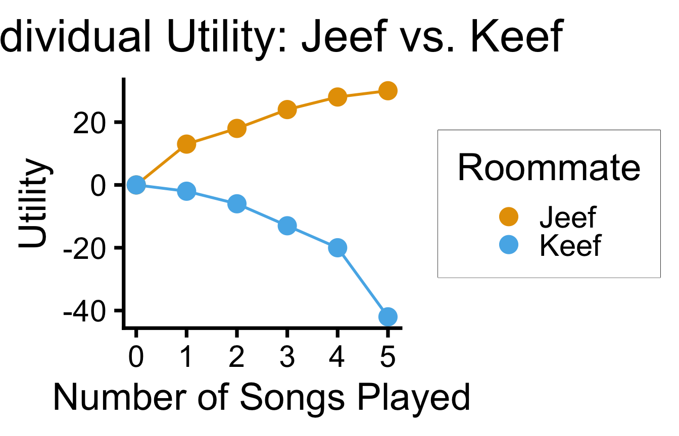
Utility \(\rightarrow\) Social Welfare with Externalities
- Jeef and Keef are roommates: Jeef loves listening to Tony Danza Tapdance Extravaganza, but Keef is normal and slowly dies inside with each additional song
library(tidyverse)
music_df <- tribble(
  ~Songs, ~Jeef, ~Keef,
  0, 0, 0,
  1, 13, -2,
  2, 18, -6,
  3, 24, -13,
  4, 28, -20,
  5, 30, -42
)
music_df <- music_df |>
  mutate(Total = Jeef + Keef)
music_df
long_df <- music_df |>
  pivot_longer(!Songs, names_to="Roommate", values_to="Utility")
util_df <- long_df |>
  filter(Roommate != "Total")
ggplot(util_df, aes(x=Songs, y=Utility, color=Roommate)) +
  geom_line(linewidth=g_linewidth) +
  geom_point(size=g_pointsize) +
  labs(
    title="Individual Utility: Jeef vs. Keef",
    x="Number of Songs Played",
    y="Utility"
  ) +
  theme_dsan("quarter")
welfare_df <- long_df |>
  filter(Roommate == "Total")
ggplot(welfare_df, aes(x=Songs, y=Utility, color=Roommate)) +
  geom_line(linewidth=g_linewidth) +
  geom_point(size=g_pointsize) +
  labs(
    title="Social Welfare: Jeef and Keef",
    x="Number of Songs Played",
    y="Social Welfare"
  ) +
  scale_color_manual(values=c(cbPalette[3]), labels=c("Total      ")) +
  theme_dsan("quarter") +
  remove_legend_title()
── Attaching core tidyverse packages ──────────────────────── tidyverse 2.0.0 ──
✔ dplyr 1.2.1 ✔ readr 2.2.0
✔ forcats 1.0.1 ✔ stringr 1.6.0
✔ lubridate 1.9.5 ✔ tibble 3.3.1
✔ purrr 1.2.1 ✔ tidyr 1.3.2
── Conflicts ────────────────────────────────────────── tidyverse_conflicts() ──
✖ dplyr::filter() masks stats::filter()
✖ dplyr::lag() masks stats::lag()
ℹ Use the conflicted package (<http://conflicted.r-lib.org/>) to force all conflicts to become errors| Songs | Jeef | Keef | Total |
|---|---|---|---|
| 0 | 0 | 0 | 0 |
| 1 | 13 | -2 | 11 |
| 2 | 18 | -6 | 12 |
| 3 | 24 | -13 | 11 |
| 4 | 28 | -20 | 8 |
| 5 | 30 | -42 | -12 |
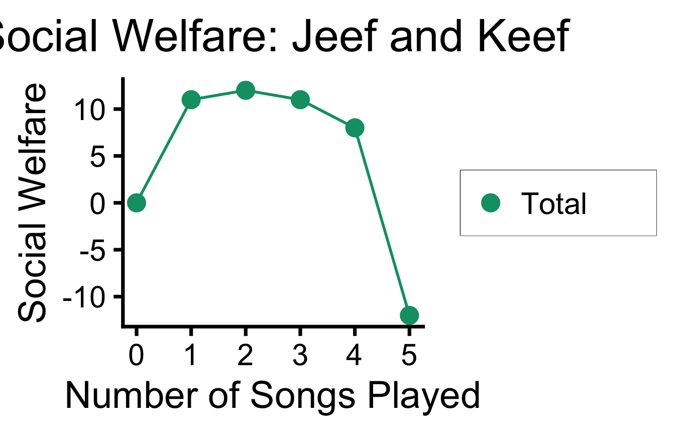
So What’s the Issue?
- These utility values are not observed
- If we try to elicit them, both Jeef and Keef have strategic incentives to lie (over-exaggerate)
- Jeef maximizes own utility by reporting \(u_j(s) = \infty\)
- (“I will literally die if I can’t listen to Lil Wayne’s ”Peanuts 2 N Elephant” prod. Lin-Manuel Miranda all day”)
- Keef maximizes own utility by reporting \(u_k(s) = -\infty\)
- (“I will literally die if I hear this elephant song again”)
- (…Quick mechanism design demo: Second price auctions)
Now with Scarce Resources
- In a given week, Jeef and Keef have 14 meals and 7 aux hours to divide amongst them
\[ \begin{align*} \max_{m_1,m_2,a_1,a_2}& W(u_1(m_1,a_1),u_2(m_2,a_2)) \\ \text{s.t. }& m_1 + m_2 \leq 14 \\ \phantom{\text{s.t. }} & ~ \, a_1 + a_2 \; \leq 7 \end{align*} \]
- Let’s assume \(u_i(m_i, a_i) = m_i + a_i\) for both
- \(\Rightarrow\) One solution: \(m_1 = 14, m_2 = 0, a_1 = 7, a_2 = 0\)…
- \(\Rightarrow\) Another: \(m_1 = 0, m_2 = 14, a_1 = 0, a_2 = 7\)…
- Who decides? Any decision implies \(\omega_1, \omega_2\) (\(\omega_1 + \omega_2 = 1\))
(Last slide = last reminder…)
Now With Moral Responsibility vs. Moral Luck!
What is the overall social welfare of a policy \(x\) (as opposed to another policy \(y\), e.g., “do nothing”)?
| Effort Class \(\rightarrow\) | \(e^{(1)}\) | \(e^{(2)}\) | \(e^{(3)}\) | \(e^{(4)}\) | \(e^{(5)}\) |
|---|---|---|---|---|---|
| Percentile Range \(\rightarrow\) | \([P_0, P_{20}]\) | \([P_{20}, P_{40}]\) | \([P_{40}, P_{60}]\) | \([P_{60}, P_{80}]\) | \([P_{80}, P_{100}]\) |
| Circumstance Class \(c^{(1)}\) | \(N_{11}\), \(W(1,1)(x)\) | \(N_{12}\), \(W(1,2)(x)\) | \(N_{13}\), \(W(1,3)(x)\) | \(N_{14}\), \(W(1,4)(x)\) | \(N_{15}\), \(W(1,5)(x)\) |
| Circumstance Class \(c^{(2)}\) | \(N_{21}\), \(W(2,1)(x)\) | \(N_{22}\), \(W(2,2)(x)\) | \(N_{23}\), \(W(2,3)(x)\) | \(N_{24}\), \(W(2,4)(x)\) | \(N_{25}\), \(W(2,5)(x)\) |
| Circumstance Class \(c^{(3)}\) | \(N_{31}\), \(W(3,1)(x)\) | \(N_{32}\), \(W(3,2)(x)\) | \(N_{33}\), \(W(3,3)(x)\) | \(N_{34}\), \(W(3,4)(x)\) | \(N_{35}\), \(W(3,5)(x)\) |
- \(N_{ij}\) = Number of people in Circumstance Class \(i\) who exert effort \(j\)
- \(W(i,j)\) = SWFL evaluated w.r.t. people in Circumstance Class \(i\) who exert effort \(j\)
Disaggregating Social Welfare: Group Representation
| Ethnic Group | Census Administrator | |||
|---|---|---|---|---|
| Bulgaria | Serbia | Greece | Turkey | |
| Bulgarian | 52.3% | 2.0% | 19.3% | 30.8% |
| Serbian | 0.0% | 71.4% | 0.0% | 3.4% |
| Greek | 10.1% | 7.0% | 37.9% | 10.6% |
| Albanian | 5.7% | 5.8% | 0.0% | 0.0% |
| Turkish | 22.1% | 8.1% | 36.8% | 51.8% |
| Other | 9.7% | 5.9% | 6.1% | 3.4% |
Estimates of ethnic composition of Macedonia, 1889-1905 (Friedman 1994)
Data-Ethical Toolkit: Implementation 👀
Code
library(tidyverse) |> suppressPackageStartupMessages()
canada_df <- tibble::tribble(
  ~Ethnicity, ~Year, ~`Percent of Total`,
  "Canadian", 1991, 3.3,
  "Canadian", 1996, 30.9,
  "Canadian", 2001, 39.4,
  "Canadian", 2006, 32.2,
  "Canadian", 2011, 32.2,
  "Canadian", 2016, 32.3,
  "Canadian", 2021, 15.6,
  "British", 1991, 20.8,
  "British", 1996, 35.9,
  "British", 2001, 33.6,
  "British", 2006, 52.8,
  "British", 2011, 34.5,
  "British", 2016, 32.5,
  "British", 2021, 42.7,
  "French", 1991, 22.8,
  "French", 1996, 19.0,
  "French", 2001, 15.8,
  "French", 2006, 16.1,
  "French", 2011, 15.5,
  "French", 2016, 13.6,
  "French", 2021, 11.0,
  "Aboriginal", 1991, 1.7,
  "Aboriginal", 1996, 3.7,
  "Aboriginal", 2001, 4.5,
  "Aboriginal", 2006, 5.5,
  "Aboriginal", 2011, 5.6,
  "Aboriginal", 2016, 6.2,
  "Aboriginal", 2021, 4.9,
)
canada_df |> ggplot(aes(x=Year, y=`Percent of Total`, color=Ethnicity)) +
  geom_point() +
  geom_line() +
  theme_dsan(base_size=24) +
  ylim(0, 60) +
  labs(title="Canadian Census Responses, 1991-2021")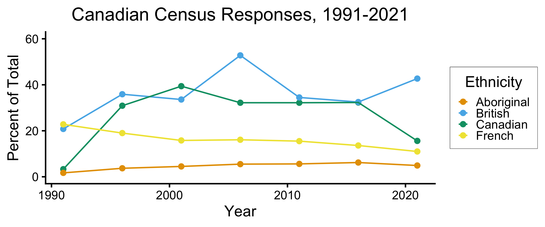
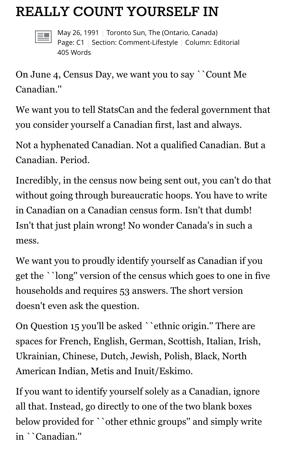
- 1991: “Count Me Canadian!” ad campaign in Toronto Sun \(\leadsto\) 3.3% write in “Canadian” \(\leadsto\) 5th largest “ethnicity” in Canada
- 1996: Legally, “Canadian” must be listed 5th in examples \(\leadsto\) 24.1% respond “Canadian” \(\leadsto\) 1st largest ethnicity
- 2001-2021: Legally, “Canadian” must be listed 1st in examples
- 2021: “French Canadian” added as option (previously recorded as two responses: “French”, “Canadian”)
Some Ethnicies with >20K Responses, 2021
Full listing (Note: None of these are aggregated into 2021 counts on previous page)
| Ethnicity | Count | % |
|---|---|---|
| Québécois | 981,635 | 2.7 |
| French Canadian | 906,315 | 2.5 |
| Caucasian (White), n.o.s. | 691,260 | 1.9 |
| European, n.o.s. | 551,910 | 1.5 |
| Jewish | 282,015 | 0.8 |
| Punjabi | 279,950 | 0.8 |
| Arab, n.o.s. | 263,710 | 0.7 |
| Asian, n.o.s. | 226,220 | 0.6 |
| Iranian | 200,465 | 0.6 |
| Christian | 200,340 | 0.6 |
| Sikh | 194,640 | 0.5 |
| Hindu | 166,160 | 0.5 |
| Mennonite | 155,095 | 0.4 |
| South Asian, n.o.s. | 120,125 | 0.3 |
| Muslim | 105,620 | 0.3 |
| Tamil | 102,170 | 0.3 |
| Ethnicity | Count | % |
|---|---|---|
| Czech | 98,925 | 0.3 |
| Black, n.o.s. | 94,585 | 0.3 |
| Newfoundlander | 91,670 | 0.3 |
| Ontarian | 80,555 | 0.2 |
| Persian | 80,340 | 0.2 |
| Slovak | 68,210 | 0.2 |
| Congolese | 45,260 | 0.1 |
| Nova Scotian | 44,720 | 0.1 |
| Czechoslovakian | 33,135 | 0.1 |
| African American | 31,430 | 0.1 |
| Yugoslavian | 30,565 | 0.1 |
| Slavic | 30,220 | 0.1 |
| Northern Irish | 25,200 | 0.1 |
| Celtic | 24,420 | 0.1 |
| Franco Ontarian | 24,110 | 0.1 |
| North American | 22,785 | 0.1 |
References
Friedman, Victor. 1994. Toward Comprehensive Peace in Southeast Europe: Conflict Prevention in the South Balkans. University of Michigan Press. https://books.google.com?id=cDJpAAAAMAAJ.
Habermas, Jürgen. 1990. Moral Consciousness and Communicative Action. MIT Press. https://books.google.com?id=fmYjgiUMy7EC.
Kasy, Maximilian, and Rediet Abebe. 2021. “Fairness, Equality, and Power in Algorithmic Decision-Making.” Proceedings of the 2021 ACM Conference on Fairness, Accountability, and Transparency (New York, NY, USA), FAccT ’21, March 1, 576–86. https://doi.org/10.1145/3442188.3445919.
Roemer, John E. 1998. Equality of Opportunity. Harvard University Press. https://books.google.com?id=2LfA_KjvOAsC.
Sen, Amartya. 1970. Collective Choice and Social Welfare: Expanded Edition. Penguin Books Limited. https://books.google.com?id=9I4sDAAAQBAJ.
Sen, Amartya. 1992. Inequality Reexamined. Clarendon Press.