# For slides
library(ggplot2)
cbPalette <- c("#E69F00", "#56B4E9", "#009E73", "#F0E442", "#0072B2", "#D55E00", "#CC79A7")
options(ggplot2.discrete.colour = cbPalette)
# Theme generator, for given sizes
theme_dsan <- function(plot_type = "full") {
    if (plot_type == "full") {
        custom_base_size <- 16
    } else if (plot_type == "half") {
        custom_base_size <- 22
    } else if (plot_type == "quarter") {
        custom_base_size <- 28
    } else {
        # plot_type == "col"
        custom_base_size <- 22
    }
    theme <- theme_classic(base_size = custom_base_size) +
        theme(
            plot.title = element_text(hjust = 0.5),
            plot.subtitle = element_text(hjust = 0.5),
            legend.title = element_text(hjust = 0.5),
            legend.box.background = element_rect(colour = "black")
        )
    return(theme)
}

knitr::opts_chunk$set(fig.align = "center")
g_pointsize <- 5
g_linesize <- 1
# Technically it should always be linewidth
g_linewidth <- 1
g_textsize <- 14

remove_legend_title <- function() {
    return(theme(
        legend.title = element_blank(),
        legend.spacing.y = unit(0, "mm")
    ))
}Week 6: Context-Sensitive Fairness
DSAN 5450: Data Ethics and Policy
Spring 2026, Georgetown University
Class Sessions
Schedule
Today’s Planned Schedule:
| Start | End | Topic | |
|---|---|---|---|
| Lecture | 3:30pm | 3:45pm | Recap: Context-Free Fairness → |
| 3:45pm | 4:00pm | Determinism \(\rightarrow\) Probability \(\rightarrow\) Causality → | |
| 4:00pm | 4:30pm | Fundamental Problem of Causal Inference → | |
| 4:30pm | 5:00pm | Do-Calculus → | |
| Break! | 5:00pm | 5:10pm | |
| 5:10pm | 6:00pm | Chalkboard Lab: DAGs for Colliders → |
Recap: Context-Free Fairness, Antecedents, and the Impossibility Result
Achieving “Fair Misclassification”
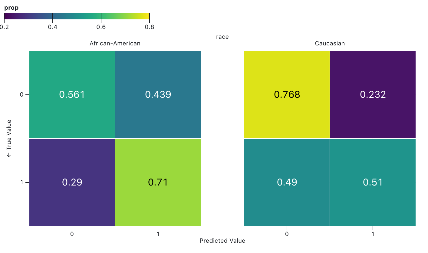
- If you think fairness = equal misclassification rates between racial groups, 👍
- If you think fairness = equal correct prediction rates between racial groups, 👎
Achieving “Fair Calibration”
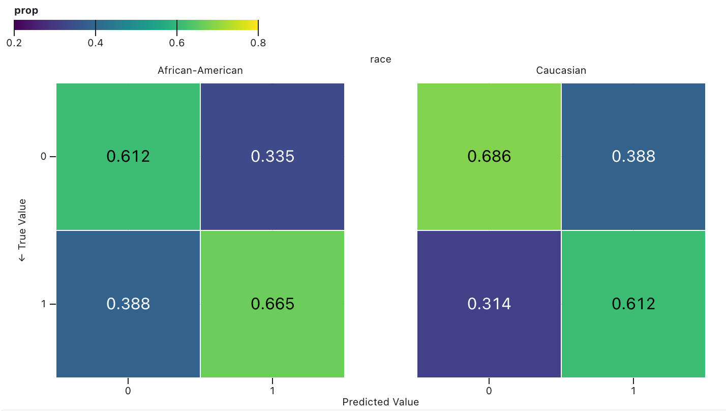
- If you think fairness = equal misclassification rates between racial groups, 👍
- If you think fairness = equal correct prediction rates between racial groups, 👎
So… What Do We Do? Option 1: Argue/Advocate
- Whitepaper(!): Berkman Klein Center for Internet & Society at Harvard University (2021), Principled Artificial Intelligence: Mapping Consensus in Ethical and Rights-based Approaches to Principles for AI
- Your first “template” for a final project!
- Problem (left til post-midterm): How do we know whose interests are included/excluded in the arguments?
- What conditions could we establish to systematically/structurally ensure inclusion of the interests of all? [Discourse ethics; coming soon!]
So… What Do We Do? Part 2: Incorporate Context
One option: argue about which of the two definitions is “better” for the next 100 years (what is the best way to give food to the poor?)
It appears to reveal an unfortunate but inexorable fact about our world: we must choose between two intuitively appealing ways to understand fairness in ML. Many scholars have done just that, defending either ProPublica’s or Northpointe’s definitions against what they see as the misguided alternative. (Simons 2023)
Another option: study and then work to ameliorate the social conditions which force us into this realm of mathematical impossibility (why do the poor have no food?)
The impossibility result is about much more than math. [It occurs because] the underlying outcome is distributed unevenly in society. This is a fact about society, not mathematics, and requires engaging with a complex, checkered history of systemic racism in the US. Predicting an outcome whose distribution is shaped by this history requires tradeoffs because the inequalities and injustices are encoded in data—in this case, because America has criminalized Blackness for as long as America has existed.
Why Not Both??
- On the one hand: yes, both! On the other hand: fallacy of the “middle ground”
- We’re back at descriptive vs. normative:
- Descriptively, given 100 values \(v_1, \ldots, v_{100}\), their mean may be a good way to summarize, if we have to choose a single number
- But, normatively, imagine that these are opinions that people hold about fairness.
- Now, if it’s the US South in 1860 and \(v_i\) represents person \(i\)’s approval of slavery, from a sample of 100 people, then approx. 97 of the \(v_i\)’s are “does not disapprove” (Rousey 2001) — in this case, normatively, is the mean \(0.97\) the “correct” answer?
- We have another case where, like the “grass is green” vs. “grass ought to be green” example, we cannot just “import” our logical/mathematical tools from the former to solve the latter! (However: this does not mean they are useless! This is the fallacy of the excluded middle, sort of the opposite of the fallacy of the middle ground)
- This is why we have ethical frameworks in the first place! Going back to Rawls: “97% of Americans think black people shouldn’t have rights” \(\nimplies\)“black people shouldn’t have rights”, since rights are a primary good
Context-Free
\(\rightarrow\) Context-Sensitive
Motivation: Linguistic Meaning
- Related to context-free vs. context-sensitive distinction in Computer Science (old-school NLP)!
- But why is it relevant to DSAN 5450?…
Impossibility Results!
- Let’s see what happens if we try to reason about definitions/meaning in language without the ability to incorporate “context” (here defined in a silly way… point holds as we go up the “language complexity hierarchy”)
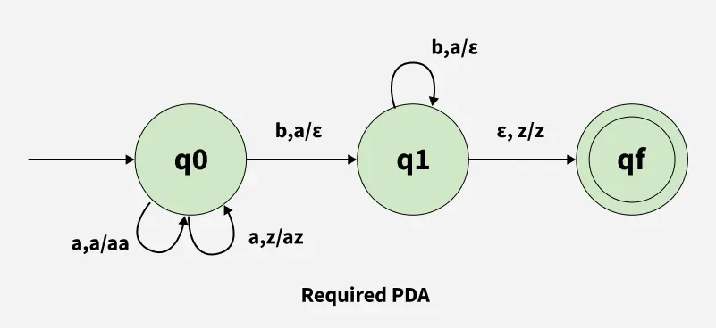
- Try to write a finite-state automata to detect “valid” strings in the language \(\{a^nb^n \mid n \in \mathbb{Z}^{\geq 0}\}\):
aabb✅,aba❌

(There is a Solution! Outside Scope of Class…)
The “Meaning” of Fairness
- Context-free (confusion-matrix-based) fairness: “plug the confusion matrix values into a formula and see if the formula is satisfied”
- Context-sensitive fairness: analyze fairness relative to a set of antecedents regarding how normative concerns should enter into our measurements of fairness
Similarity-Based Fairness
Group Fairness \(\rightarrow\) Individual Fairness
- The crucial insight of Dwork: group-level fairness does not ensure that individuals are treated fairly as individuals
- Exactly the issue we’ve seen with utilitarianism: optimizing society-level “happiness” may lead to individuals being brutally mistreated (e.g., having their rights violated)
- So, at a high level, Dwork’s proposal could provide a Rawls-style ordering: individual fairness lexically prior to group-level fairness (optimize group-level fairness once individual-level is satisfied)
The (Normative!) Antecedent
- Not well-liked in industry / policy because you can’t just “plug in” results of your classifier and get True/False “we satisfied fairness!” …But this is exactly the point!

Bringing In Context
- In itself, the principle of equal treatment is abstract, a formal relationship that lacks substantive content”
- The principle must be given content by defining which cases are similar and which are different, and by considering what kinds of differences justify differential treatment
- Deciding what differences are relevant, and what kinds of differential treatment are justified by particular differences, requires wrestling with moral and political debates about the responsibilities of different institutions to address persistent injustice (Simons 2023, 51)
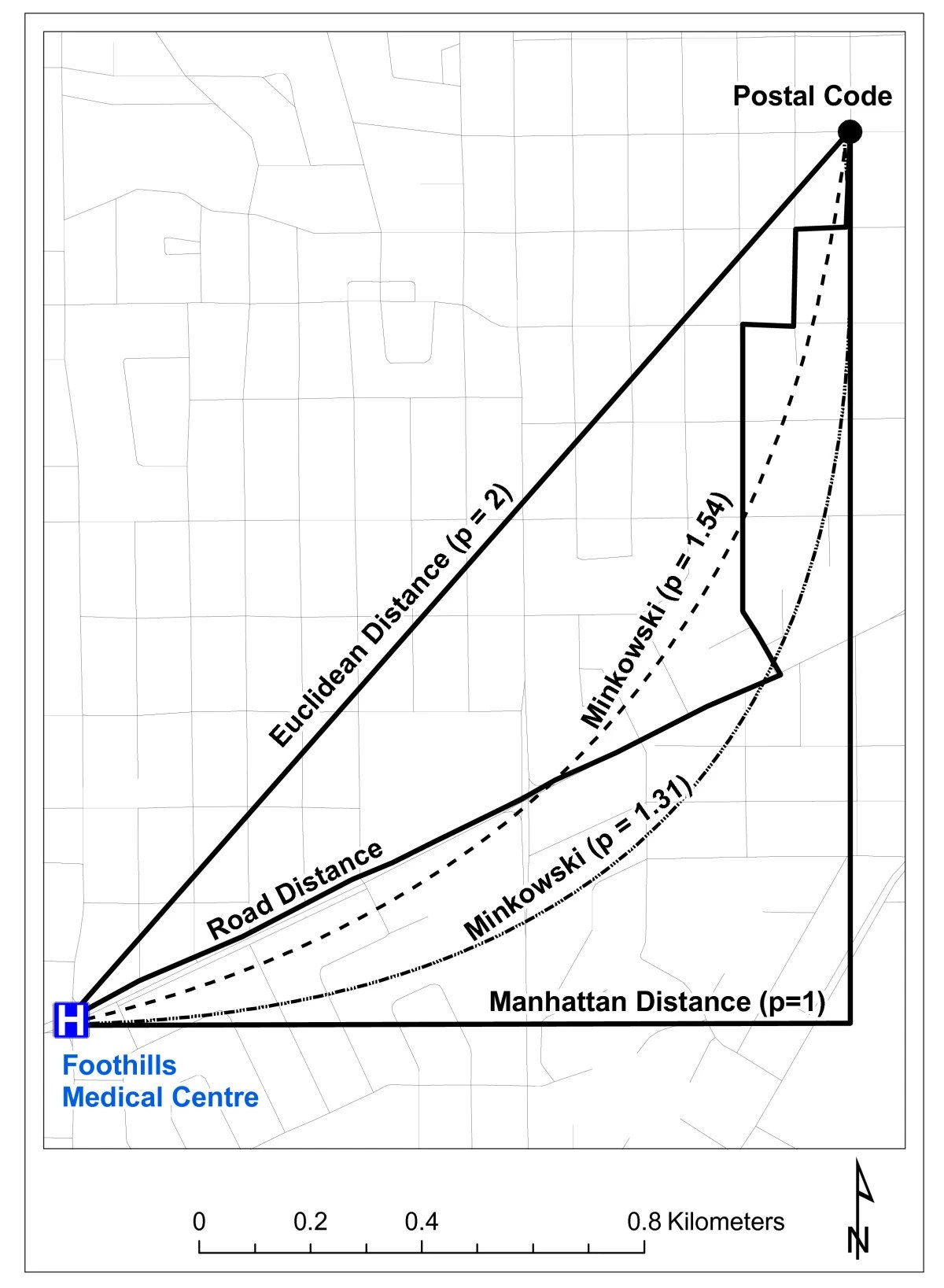
Remember Distance Metrics?(!)
- A core element in both similarity-based and causal fairness!
- Already difficult to choose a metric on pragmatic grounds (ambulance needs to get to hospital)
- Now people will also have fundamental normative disagreements about what should and should not determine difference
Satisfying Individual vs. Group Fairness
An algorithm is individually fair if, for all individuals \(x\) and \(y\), we have
\[ \textsf{dist}(r(x), r(y)) \leq \textsf{dist}(x, y) \]
\(\implies\) an advertising system must show similar sets of ads to similar users.
It achieves group fairness-through-parity for two groups of users \(S\) and \(T\) when:
\[ \textsf{dist}(\mathbb{E}_{s \in S}[r(s)], \mathbb{E}_{t \in T}[r(t)]) \leq \varepsilon \]
where \(\mathbb{E}_{s \in S}\) and \(\mathbb{E}_{t \in T}\) denote the expectation of ads seen by an individual chosen uniformly among \(S\) and \(T\). This definition implies that the difference in probability between two groups of seeing a particular ad will be bounded by \(\varepsilon\).
Given these definitions: Individual fairness \(\nimplies\) group fairness, and vice versa! (Riederer and Chaintreau 2017)
The Importance of Not Excluding Race!
- On HW2 you will see how, on the one hand: excluding race from the similarity metric ensures race-blind fairness
- But, on the other hand: race-blind fairness can not only maintain but also amplify preexisting inequalities
- By including race in our similarity metric, we can explicitly take this into account!
- Ex: someone with a (morally irrelevant) disadvantage due to birth lottery who achieves an SAT score of 1400 is similar to someone with a (morally irrelevant) advantage due to birth lottery who achieves an SAT score of 1500
Equality of Opportunity
- This notion (last bullet of the previous slide) is contentious, to say the least
- But also, crucially: our job is not to decide the similarity metric unilaterally!
- The equality of opportunity approach is not itself a similarity metric!
- It is a “meta-algorithm” for translating normative positions (consequents of an ethical framework) into concrete fairness constraints that you can then impose on ML algorithms

Roemer’s Algorithm
- Equality of Opportunity algorithm boils down to (Input 0 = data on individuals \(X_i\)):
- Input 1 (!): Attributes \(J_{\text{advantage}} \subseteq X_i\) that a society (real or hypothetical) considers normatively relevant for an outcome, but that people are not individually responsible for (e.g., race or nationality via birth lottery)
- Input 2: Attributes \(J_{\text{merit}} \subseteq X_i\) that a society considers people individually responsible for (effort, sacrificing short-term pleasure for longer-term benefits, etc.)
- : Set of individuals in society \(S\) is partitioned into subsets \(S_i\), where \(i\) is some combination of particular values for the attributes in \(X_{\text{advantage}}\)
- : Individuals’ context-sensitive scores are computed relative to their group \(S_i\), as percentile of their \(X_{\text{merit}}\) value relative to distribution of \(X_{\text{merit}}\) values across \(S_i\)
- Outcome: Now that we have incorporated social context, by converting the original context-free units (e.g., numeric SAT score) into context-sensitive units (percentile of numeric SAT score within distribution of comparable individuals), we can compare people across groups on the basis of context-sensitive scores!
An Overly-Simplistic Example (More on HW2!)
- \(\mathbf{x}_i = (x_{i,1}, x_{i,2}, x_{i,3}) = (\texttt{wealth}_i, \texttt{study\_hrs}_i, \texttt{SAT}_i)\)
- \(J_{\text{advantage}} = (1) = (\texttt{wealth})\), \(J_{\text{merit}} = (2) = (\texttt{study\_hrs})\)
- \(\Rightarrow \texttt{study\_hrs} \rightarrow \texttt{SAT}\) a “fair” pathway
- \(\Rightarrow \texttt{wealth} \rightarrow \texttt{SAT}\) an “unfair” pathway
- \(\Rightarrow\) School admission decisions “fair” to the extent that they capture the direct effect \(\texttt{study\_hrs} \rightarrow \texttt{SAT} \rightarrow \texttt{admit}\), but aren’t affected by indirect effect \(\texttt{wealth} \rightarrow \texttt{SAT} \rightarrow \texttt{admit}\)
At a Macro Level!

Causal Fairness
The State of the Art!
- Current state of fairness in AI: measures which explicitly model causal connections between variables of interest are most promising for robust notions of fairness
- Robust in the sense of:
- Being normatively desirable (as in, matching the key tenets of our ethical frameworks) while also being
- Descriptively tractable (as in, concretely implementable in math/code, and transparent enough to allow us to evaluate and update these implementations, using a process like reflective equilibrium).
The Antecedent
- Since it’s impossible to eliminate information about sensitive attributes like race/gender/etc. from our ML algorithms…
- Fairness should instead be defined on the basis of how this sensitive information “flows” through the causal chain of decisions which lead to an given (observed) outcome
The New Object of Analysis: Causal Pathways
- Once we have a model of the causal connections among:
- Variables that we care about socially/normatively, and
- Variables used by a Machine Learning algorithm,
- We can then use techniques developed by statisticians who study causal inference to
- Block certain “causal pathways” that we deem normatively unjustifiable while allowing other pathways that we deem to be normatively justifiable.
Causal Fairness in HW2
- Intuition required to make the jump from correlational approach (from statistics and probability generally, and DSAN 5100 specifically!) to causal approach!
- Causal approach builds on correlational, but…
- Stricter, directional standard for \(X \rightarrow Y\)
- Easy cases: find high correlation \(|\text{corr}(X,Y)|\), embed in a causal diagram, evaluate \(\Pr(Y \mid \text{do}(X)) \overset{?}{>} \Pr(Y \mid \neg\text{do}(X))\)
- Hard cases: can have \(\Pr(Y \mid \text{do}(X)) \overset{?}{>} \Pr(Y \mid \neg\text{do}(X))\) even when \(\text{corr}(X,Y) = 0\) 😰 (dw, we’ll get there!)
Causal Building Blocks
- DSAN 5100 precedent: nodes in the network \(X\), \(Y\) are Random Variables, connections \(X \leftrightarrow Y\) are joint distributions \(\Pr(X, Y)\)
- Directional edges \(X \rightarrow Y\), then, just represent conditional distributions: \(X \rightarrow Y\) is \(\Pr(Y \mid X)\)
- Where we’re going: connections \(X \leftrightarrow Y\) represent unknown but extant causal connections between \(X\) and \(Y\), while \(X \rightarrow Y\) represents a causal relationship between \(X\) and \(Y\)
- Specifically, \(X \rightarrow Y\) now means: an intervention that changes the value of \(X\) by \(\varepsilon\) causes a change in the value of \(Y\) by \(f(\varepsilon)\)
What Is To Be Done?

Face Everything And Rise: Controlled, Randomized Experiment Paradigm
- Find good comparison cases: Treatment and Control
- Without a control group, you cannot make inferences!
- Selecting on the dependent variable…
Selecting on the Dependent Variable
- Jeff’s rant: If you care about actually solving social issues, this should infuriate you
Complications: Selection
- Tldr: Why did this person (unit) end up in the treatment group? Why did this other person (unit) end up in the control group?
- Are there systematic differences?
- Vietnam/Indochina Draft: Why can’t we just study [men who join the military] versus [men who don’t], and take the difference as a causal estimate?
Complications: Compliance
- We want people assigned to treatment to take the treatment, and people assigned to control to take the control
- “Compliance”: degree to which this is true in experiment
- High compliance = most people actually took what they were assigned
- Low compliance = lots of people who were assigned to treatment actually took control, and vice-versa
- What problems might exist w.r.t compliance in the Draft?
Next Week and HW2: Experimental \(\rightarrow\) Observational Data
- In observational studies, researchers have no control over assignment to treatment/control 😨
- On the one hand… Forget Everything And Run [to randomized, controlled experiments], if you can.
- On the other hand… statisticians over the last 4 centuries have developed fancy causal inference tools/techniques to help us Face Everything And Rise 🧐
For Now: Matching
- In a randomized, controlled experiment, we can ensure (since we have control over the assignment mechanism) that the only systematic difference between \(C\) and \(T\) is that \(T\) received the treatment and \(C\) did not
- In an observational study, we “show up too late”!
- Thus, we no longer refer to assignment but to selection
- And, our job is to figure out (reverse engineer!) the selection mechanism, then correct for its non-randomness: basically, we “transform” from observational to experimental setting through weighting (👀 W02)
Quick Clarifications / Recaps!
Clarification: Ecological Inference
- I gave the worst example for this: generalizing from population to single person (white people \(\rightarrow\) Jeff)!
- As Trey helpfully pointed out, this is the “obvious” fallacy of stereotyping a person based on group membership
- In reality, the “ecological fallacy” is more subtly (but just as fallacious-ly) committed from aggregate to slightly-less-aggregate populations!
- Example: DC Public Schools vs. Jackson-Reed
Eureka Moment (for Midterm Prep Purposes)
- I totally forgot to mention: John Stuart Mill, the progenitor of what we today identify as utilitarianism, was himself tortured mercilessly, by his father John Mill (bffs with Jeremy Bentham) for the “greater good of society”!

Blasting Off Into Causality!
DGPs and the Emergence of Order
- Who can guess the state of this process after 10 steps, with 1 person?
- 10 people? 50? 100? (If they find themselves on the same spot, they stand on each other’s heads)
- 100 steps? 1000?

The Result: 16 Steps
Code
library(tibble)
library(ggplot2)
library(ggExtra)
library(dplyr)
Attaching package: 'dplyr'The following objects are masked from 'package:stats':
filter, lagThe following objects are masked from 'package:base':
intersect, setdiff, setequal, unionCode
library(tidyr)
# From McElreath!
gen_histo <- function(reps, num_steps) {
  support <- c(-1,1)
  pos <-replicate(reps, sum(sample(support,num_steps,replace=TRUE,prob=c(0.5,0.5))))
  #print(mean(pos))
  #print(var(pos))
  pos_df <- tibble(x=pos)
  clt_distr <- function(x) dnorm(x, 0, sqrt(num_steps))
  plot <- ggplot(pos_df, aes(x=x)) +
    geom_histogram(aes(y = after_stat(density)), fill=cbPalette[1], binwidth = 2) +
    stat_function(fun = clt_distr) +
    theme_dsan("quarter") +
    theme(title=element_text(size=16)) +
    labs(
      title=paste0(reps," Random Walks, ",num_steps," Steps")
    )
  return(plot)
}
gen_walkplot <- function(num_people, num_steps, opacity=0.15) {
  support <- c(-1, 1)
  # Unique id for each person
  pid <- seq(1, num_people)
  pid_tib <- tibble(pid)
  pos_df <- tibble()
  end_df <- tibble()
  all_steps <- t(replicate(num_people, sample(support, num_steps, replace = TRUE, prob = c(0.5, 0.5))))
  csums <- t(apply(all_steps, 1, cumsum))
  csums <- cbind(0, csums)
  # Last col is the ending positions
  ending_pos <- csums[, dim(csums)[2]]
  end_tib <- tibble(pid = seq(1, num_people), endpos = ending_pos, x = num_steps)
  # Now convert to tibble
  ctib <- as_tibble(csums, name_repair = "none")
  merged_tib <- bind_cols(pid_tib, ctib)
  long_tib <- merged_tib %>% pivot_longer(!pid)
  # Convert name -> step_num
  long_tib <- long_tib %>% mutate(step_num = strtoi(gsub("V", "", name)) - 1)
  # print(end_df)
  grid_color <- rgb(0, 0, 0, 0.1)

  # And plot!
  walkplot <- ggplot(
      long_tib,
      aes(
          x = step_num,
          y = value,
          group = pid,
          # color=factor(label)
      )
  ) +
      geom_line(linewidth = g_linesize, alpha = opacity, color = cbPalette[1]) +
      geom_point(data = end_tib, aes(x = x, y = endpos), alpha = 0) +
      scale_x_continuous(breaks = seq(0, num_steps, num_steps / 4)) +
      scale_y_continuous(breaks = seq(-20, 20, 10)) +
      theme_dsan("quarter") +
      theme(
          legend.position = "none",
          title = element_text(size = 16)
      ) +
      theme(
          panel.grid.major.y = element_line(color = grid_color, linewidth = 1, linetype = 1)
      ) +
      labs(
          title = paste0(num_people, " Random Walks, ", num_steps, " Steps"),
          x = "Number of Steps",
          y = "Position"
      )
}
wp1 <- gen_walkplot(500, 16, 0.05)
Warning: The `x` argument of `as_tibble.matrix()` must have unique column names if
`.name_repair` is omitted as of tibble 2.0.0.
ℹ Using compatibility `.name_repair`.Code
ggMarginal(wp1, margins = "y", type = "histogram", yparams = list(binwidth = 1))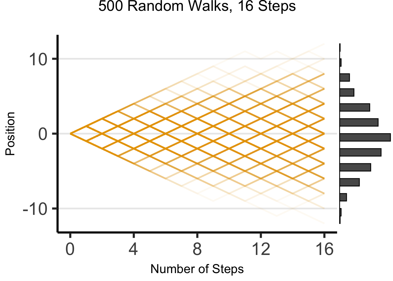
The Result: 64 Steps
Code
library(ggExtra)
wp2 <- gen_walkplot(5000,64,0.008) +
  ylim(-30,30)
Scale for y is already present.
Adding another scale for y, which will replace the existing scale.Code
ggMarginal(wp2, margins = "y", type = "histogram", yparams = list(binwidth = 1))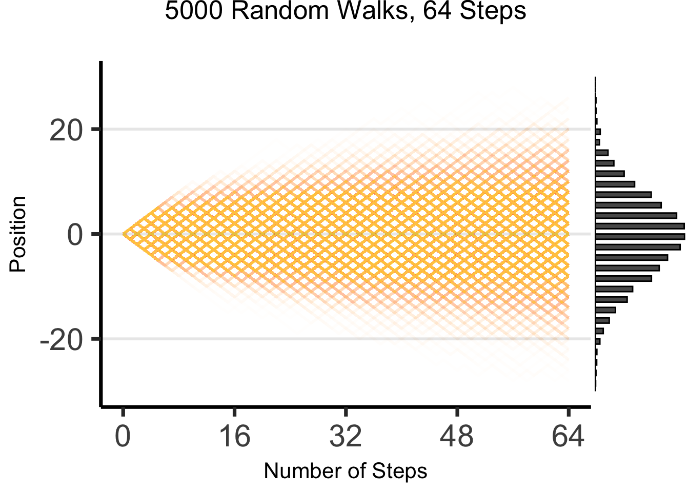
“Mathematical/Scientific Modeling”
- Thing we observe (poking out of water): data
- Hidden but possibly discoverable through deeper investigation (ecosystem under surface): model / DGP

So What’s the Problem?
- Non-probabilistic models: High potential for being garbage
- tldr: even if SUPER certain, using \(\Pr(\mathcal{H}) = 1-\varepsilon\) with tiny \(\varepsilon\) has literal life-saving advantages (Finetti 1972)
- Probabilistic models: Getting there, still looking at “surface”
- Of the \(N = 100\) times we observed event \(X\) occurring, event \(Y\) also occurred \(90\) of those times
- \(\implies \Pr(Y \mid X) = \frac{\#[X, Y]}{\#[X]} = \frac{90}{100} = 0.9\)
- Causal models: Does \(Y\) happen because of \(X\) happening? For that, need to start modeling what’s happening under the surface making \(X\) and \(Y\) “pop up” together so often
Causal Inference
The Intuitive But Boring Problem of Causal Inference
library(dplyr)
library(ggplot2)
ga_lawyers <- c(21362, 22254, 23134, 23698, 24367, 24930, 25632, 26459, 27227, 27457)
ski_df <- tibble::tribble(
  ~year, ~varname, ~value,
  2000, "ski_revenue", 1551,
  2001, "ski_revenue", 1635,
  2002, "ski_revenue", 1801,
  2003, "ski_revenue", 1827,
  2004, "ski_revenue", 1956,
  2005, "ski_revenue", 1989,
  2006, "ski_revenue", 2178,
  2007, "ski_revenue", 2257,
  2008, "ski_revenue", 2476,
  2009, "ski_revenue", 2438,
)
ski_mean <- mean(ski_df$value)
ski_sd <- sd(ski_df$value)
ski_df <- ski_df %>% mutate(val_scaled = 12*value, val_norm = (value - ski_mean)/ski_sd)
law_df <- tibble::tibble(year=2000:2009, varname="ga_lawyers", value=ga_lawyers)
law_mean <- mean(law_df$value)
law_sd <- sd(law_df$value)
law_df <- law_df %>% mutate(val_norm = (value - law_mean)/law_sd)
spur_df <- dplyr::bind_rows(ski_df, law_df)
ggplot(spur_df, aes(x=year, y=val_norm, color=factor(varname, labels = c("Ski Revenue","Lawyers in Georgia")))) +
  stat_smooth(method="loess", se=FALSE) +
  geom_point(size=g_pointsize/1.5) +
  labs(
    fill="",
    title="Ski Revenue vs. Georgia Lawyers",
    x="Year",
    color="Correlation: 99.2%",
    linetype=NULL
  ) +
  theme_dsan() +
  scale_x_continuous(
    breaks=seq(from=2000, to=2014, by=2)
  ) +
  #scale_y_continuous(
  #  name="Total Revenue, Ski Facilities (Million USD)",
  #  sec.axis = sec_axis(~ . * law_sd + law_mean, name = "Number of Lawyers in Georgia")
  #) +
  scale_y_continuous(breaks = -1:1,
    labels = ~ . * round(ski_sd,1) + round(ski_mean,1),
    name="Total Revenue, Ski Facilities (Million USD)",
    sec.axis = sec_axis(~ . * law_sd + law_mean, name = "Number of Lawyers in Georgia")) +
  expand_limits(x=2010) +
  #geom_hline(aes(yintercept=x, color="Mean Values"), as.data.frame(list(x=0)), linewidth=0.75, alpha=1.0, show.legend = TRUE) +
  scale_color_manual(
    breaks=c('Ski Revenue', 'Lawyers in Georgia'),
    values=c('Ski Revenue'=cbPalette[1], 'Lawyers in Georgia'=cbPalette[2])
  )
Ignoring unknown labels:
• fill : ""
`geom_smooth()` using formula = 'y ~ x'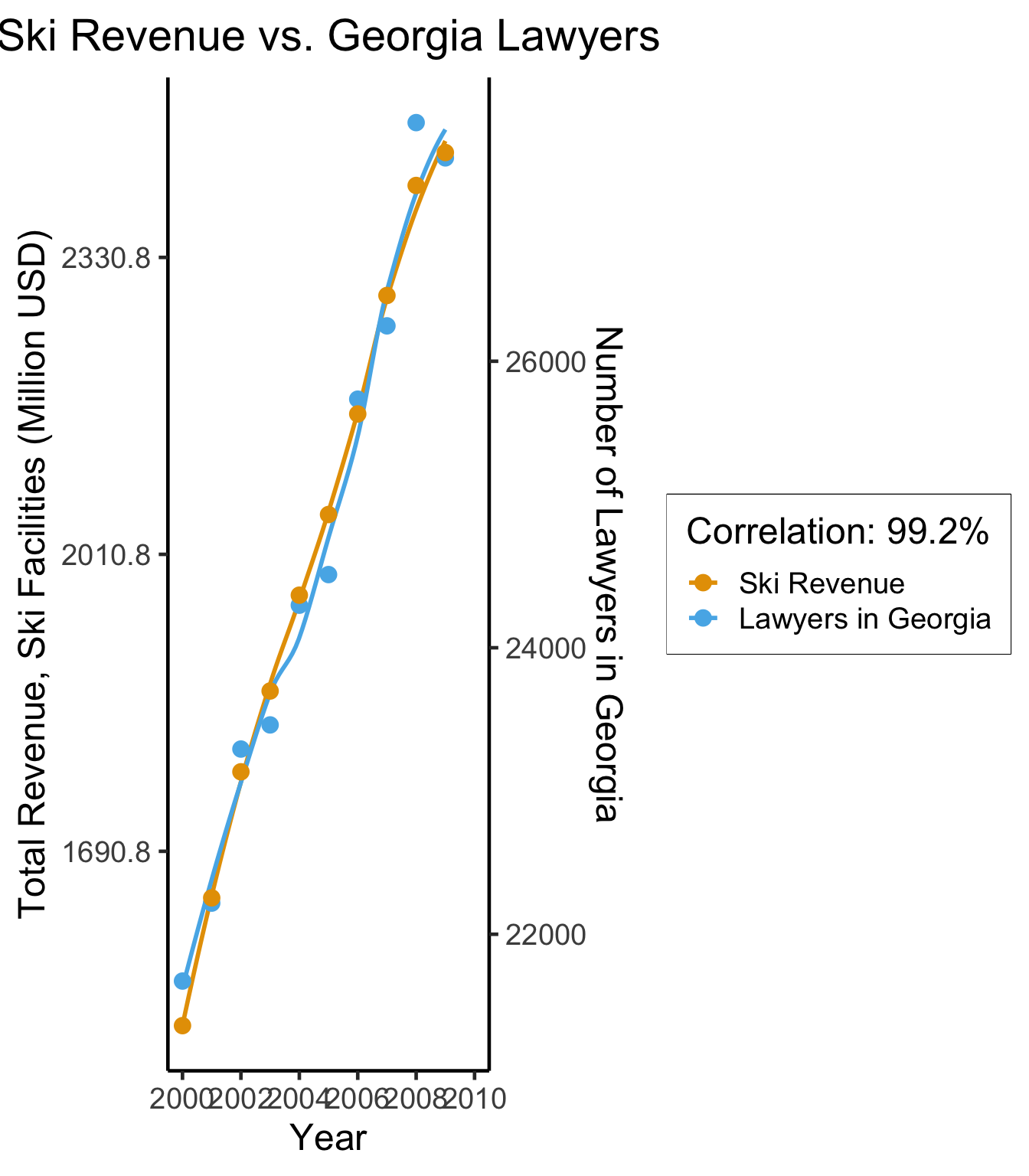
cor(ski_df$value, law_df$value)[1] 0.9921178(Based on Spurious Correlations, Tyler Vigen)
- This, however, is only a mini-boss. Beyond it lies the truly invincible FINAL BOSS… 🙀
The Fundamental Problem of Causal Inference
The only workable definition of “\(X\) causes \(Y\)”:
- The problem? We live in one world, not two identical worlds simultaneously 😭
What Is To Be Done?
Face Everything And Rise: Controlled, Randomized Experiment Paradigm
- Find good comparison cases: Treatment and Control
- Without a control group, you cannot make inferences!
- Selecting on the dependent variable…
Selecting on the Dependent Variable
- Jeff’s ABHYSIOWDCI claim: If we care about intervening to reduce social ills, this literally has negative value (Goes up to zero value if you don’t publish it though! 😉)
(Annoying But Hopefully You’ll See the Importance Once We Digest Causal Inference… a standard term in The Sciences)
Complications: Selection
- Tldr: Why did this person (unit) end up in the treatment group? Why did this other person (unit) end up in the control group?
- Are there systematic differences?
- “““Vietnam”“” “““War”“” Draft: Why can’t we just study [men who join the military] versus [men who don’t], and take the difference as a causal estimate?
The Solution: Matching
(W02 we looked at propensity score matching… kind of the Naïve Bayes of matching)
- Controlled experiment: we can ensure (since we have control over the assignment mechanism) the only systematic difference between \(C\) and \(T\) is: \(T\) received treatment, \(C\) did not
- In an observational study, we’re “too late”! Thus, we no longer refer to assignment but to selection
- Our job is to reverse engineer the selection mechanism, then correct for its non-randomness. Spoiler: “transform” observational \(\rightarrow\) experimental via weighting.
- That’s the gold at end of rainbow. The rainbow itself is…
Do-Calculus
Our Data-Generating Process
- \(Y\): Future success, \(\mathcal{R}_Y = \{0, 1\}\)
- \(E\): Private school education, \(\mathcal{R}_E = \{0, 1\}\)
- \(V\): Born into poverty, \(\mathcal{R}_V = \{0, 1\}\)
NoteThe Private School \(\leadsto\) Success Pipeline 🤑
- Sample independent RVs \(U_1 \sim \mathcal{B}(1/2)\), \(U_2 \sim \mathcal{B}(1/3)\), \(U_3 \sim \mathcal{B}(1/3)\)
- \(V \leftarrow U_1\)
- \(E \leftarrow \textsf{if }(V = 1)\textsf{ then } 0\textsf{ else }U_2\)
- \(Y \leftarrow \textsf{if }(V = 1)\textsf{ then }0\textsf{ else }U_3\)
Chalkboard Time…
- \(\Pr(Y = 1) = \; ?\)
- \(\Pr(Y = 1 \mid E = 1) = \; ?\)

Top Secret Answers Slide (Don’t Peek)
- \(\Pr(Y = 1) = \frac{1}{6}\)
- \(\Pr(Y = 1 \mid E = 1) = \frac{1}{3}\)
- \(\overset{✅}{\implies}\) One out of every three private-school graduates is successful, vs. one out of every six graduates overall
- \(\overset{❓}{\implies}\) Private school doubles likelihood of success!
- Latter is only true if intervening/changing/doing \(E = 0 \leadsto E = 1\) is what moves \(\Pr(Y = 1)\) from \(\frac{1}{6}\) to \(\frac{1}{3}\)!
Chalkboard Time 2: Electric Boogaloo
- \(\Pr(Y = 1) = \frac{1}{6}\)
- \(\Pr(Y = 1 \mid E = 1) = \frac{1}{3}\)
- \(\Pr(Y = 1 \mid \textsf{do}(E = 1)) = \; ?\)
- Here, \(\textsf{do}(E = 1)\) means diving into the DGP below the surface and changing it so \(E = 1\)… Setting \(E\) to be \(1\)
Note\(\text{DGP}(Y \mid \textsf{do}(E = 1))\)
- Sample independent RVs \(U_1 \sim \mathcal{B}(1/2)\), \(U_2 \sim \mathcal{B}(1/3)\), \(U_3 \sim \mathcal{B}(1/3)\)
- \(V \leftarrow U_1\)
- \(E \leftarrow \textsf{if }(V = 1)\textsf{ then } 0\textsf{ else }U_2\)
- \(Y \leftarrow \textsf{if }(V = 1)\textsf{ then }0\textsf{ else }U_3\)
Double Quadruple Secret Answer Slide
- \(\Pr(Y = 1) = \frac{1}{6}\)
- \(\Pr(Y = 1 \mid E = 1) = \frac{1}{3}\)
- \(\Pr(Y = 1 \mid \textsf{do}(E = 1)) = \frac{1}{6}\)
- The takeaway:
- \(\Pr(Y = 1 \mid E = 1) < \Pr(Y = 1)\), but
- \(\Pr(Y = 1 \mid \textsf{do}(E = 1)) = \Pr(Y = 1)\)
The Problem of Colliders
- \(X\) and \(Y\) are diseases which occur independently, no interrelationship, with probability \(1/3\)
- Either \(X\) or \(Y\) sufficient for admission to hospital, \(Z\)
- We have: \(X \rightarrow Z \leftarrow Y\) [🚨 Collider alert!]

What’s the Issue?
If we only have data on patients (\(Z = 1\)), observing \(X = 1\) lowers \(\Pr(Y = 1)\), despite the fact that \(X \perp Y\)!
\(X \perp Y\), but \((X \not\perp Y) \mid Z\)
The moral: controlling for stuff does not necessarily solve problem of causal inference, and can actually make it worse (inducing correlations where they don’t actually exist) 😭


The Causal Trinity: When Controlling for Stuff Helps
- Fork: Controlling helps!
- Confounder: Controlling helps!
- Collider: Controlling makes things worse 😞
The Final Diagrammatic Boss: SWIGs
- Single World Intervention Graphs


References
Dwork, Cynthia, Moritz Hardt, Toniann Pitassi, Omer Reingold, and Rich Zemel. 2011. “Fairness Through Awareness.” Pre-published November 28. https://doi.org/10.48550/arXiv.1104.3913.
Finetti, Bruno de. 1972. Probability, Induction and Statistics: The Art of Guessing. J. Wiley. https://books.google.com?id=hENg7qRPOPYC.
Firth, John Rupert. 1968. Selected Papers of J.R. Firth, 1952-59. Longmans. https://books.google.com?id=Uxu3AAAAIAAJ.
Hume, David. 1739. A Treatise of Human Nature: Being an Attempt to Introduce the Experimental Method of Reasoning Into Moral Subjects; and Dialogues Concerning Natural Religion. Longmans, Green.
Kiat, Lim Swee. 2018. “Machines Gone Wrong.” Singapore University of Technology and Design. https://machinesgonewrong.com/about/.
Riederer, Christopher, and Augustin Chaintreau. 2017. “The Price of Fairness in Location Based Advertising.” Fairness, Accountability, and Transparency Workshop on Responsible Recommendation, ahead of print. https://doi.org/10.18122/B2MD8C.
Roemer, John E. 1998. Equality of Opportunity. Harvard University Press. https://books.google.com?id=2LfA_KjvOAsC.
Rousey, Dennis C. 2001. “Friends and Foes of Slavery: Foreigners and Northerners in the Old South.” Journal of Social History 35 (2): 373–96. https://www.jstor.org/stable/3790193.
Shahid, Rizwan, Stefania Bertazzon, Merril L. Knudtson, and William A. Ghali. 2009. “Comparison of Distance Measures in Spatial Analytical Modeling for Health Service Planning.” BMC Health Services Research 9 (1): 200. https://doi.org/10.1186/1472-6963-9-200.
Simons, Josh. 2023. Algorithms for the People: Democracy in the Age of AI. Princeton University Press. https://books.google.com?id=hIKIEAAAQBAJ.