# For slides
library(ggplot2)
cbPalette <- c("#E69F00", "#56B4E9", "#009E73", "#F0E442", "#0072B2", "#D55E00", "#CC79A7")
options(ggplot2.discrete.colour = cbPalette)
# Theme generator, for given sizes
theme_dsan <- function(plot_type = "full") {
    if (plot_type == "full") {
        custom_base_size <- 16
    } else if (plot_type == "half") {
        custom_base_size <- 22
    } else if (plot_type == "quarter") {
        custom_base_size <- 28
    } else {
        # plot_type == "col"
        custom_base_size <- 22
    }
    theme <- theme_classic(base_size = custom_base_size) +
        theme(
            plot.title = element_text(hjust = 0.5),
            plot.subtitle = element_text(hjust = 0.5),
            legend.title = element_text(hjust = 0.5),
            legend.box.background = element_rect(colour = "black")
        )
    return(theme)
}

knitr::opts_chunk$set(fig.align = "center")
g_pointsize <- 5
g_linesize <- 1
# Technically it should always be linewidth
g_linewidth <- 1
g_textsize <- 14

remove_legend_title <- function() {
    return(theme(
        legend.title = element_blank(),
        legend.spacing.y = unit(0, "mm")
    ))
}Week 6: Context-Sensitive Fairness
DSAN 5450: Data Ethics and Policy
Spring 2026, Georgetown University
Wednesday, February 18, 2026
Achieving “Fair Misclassification”
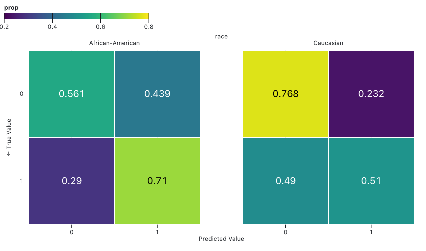
- If you think fairness = equal misclassification rates between racial groups, 👍
- If you think fairness = equal correct prediction rates between racial groups, 👎
Achieving “Fair Calibration”
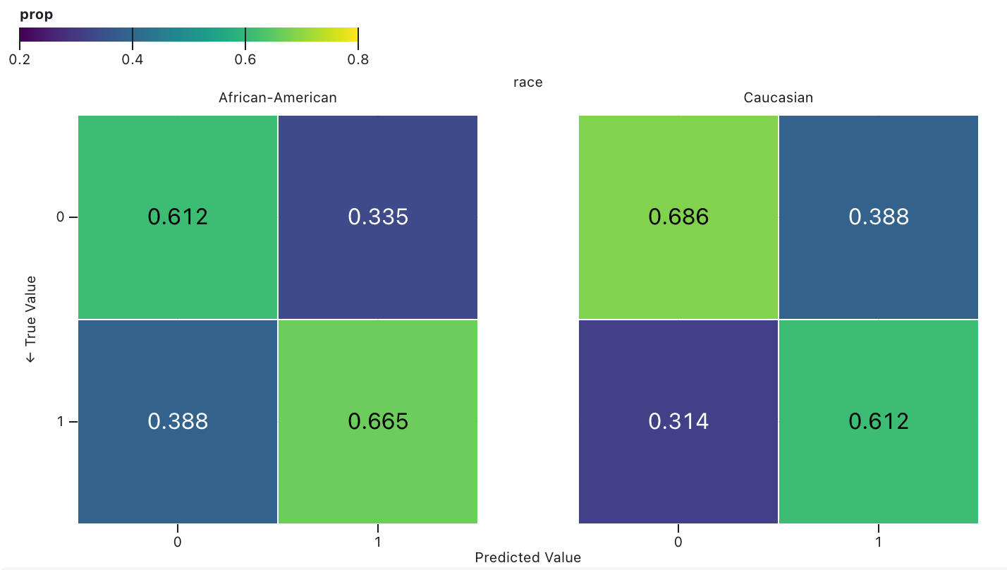
- If you think fairness = equal misclassification rates between racial groups, 👍
- If you think fairness = equal correct prediction rates between racial groups, 👎
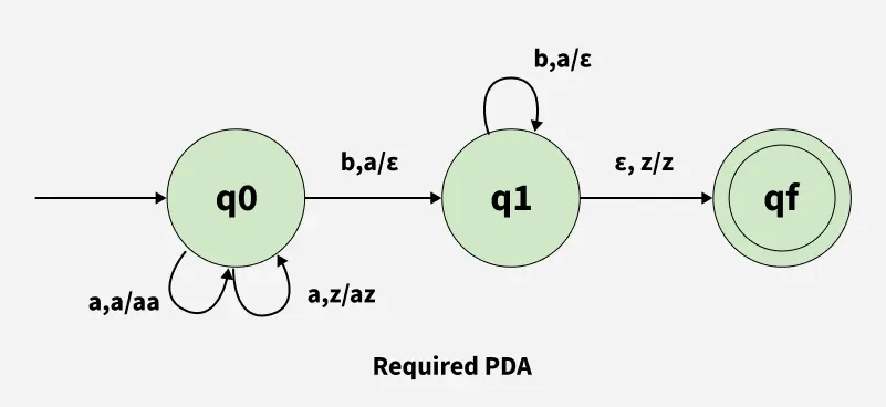
Impossibility Results!
- Let’s see what happens if we try to reason about definitions/meaning in language without the ability to incorporate “context” (here defined in a silly way… point holds as we go up the “language complexity hierarchy”)
- Try to write a finite-state automata to detect “valid” strings in the language \(\{a^nb^n \mid n \in \mathbb{Z}^{\geq 0}\}\):
aabb✅,aba❌

(There is a Solution! Outside Scope of Class…)
The (Normative!) Antecedent
- Not well-liked in industry / policy because you can’t just “plug in” results of your classifier and get True/False “we satisfied fairness!” …But this is exactly the point!

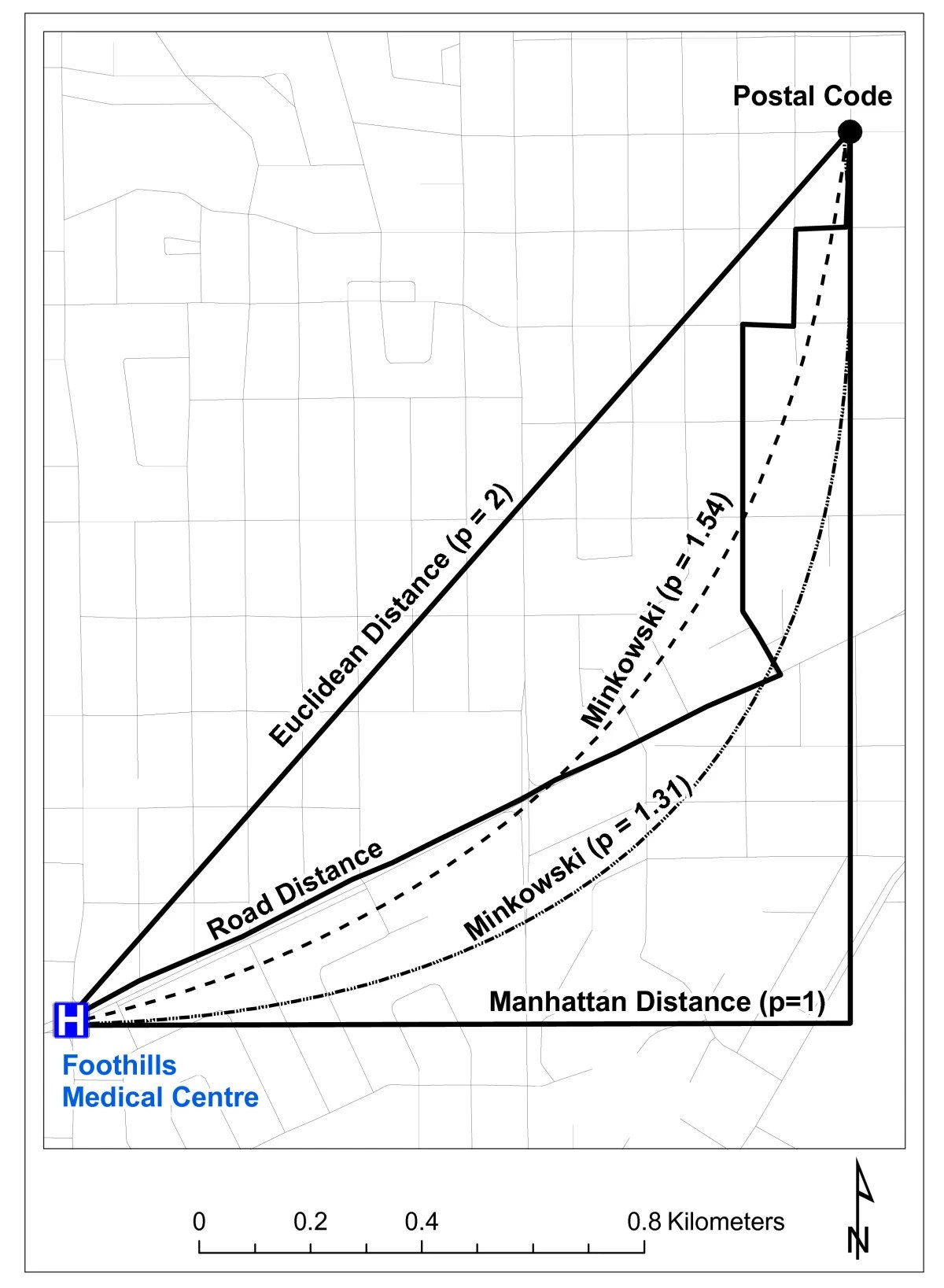
Remember Distance Metrics?(!)
- A core element in both similarity-based and causal fairness!
- Already difficult to choose a metric on pragmatic grounds (ambulance needs to get to hospital)
- Now people will also have fundamental normative disagreements about what should and should not determine difference
Equality of Opportunity
- This notion (last bullet of the previous slide) is contentious, to say the least
- But also, crucially: our job is not to decide the similarity metric unilaterally!
- The equality of opportunity approach is not itself a similarity metric!
- It is a “meta-algorithm” for translating normative positions (consequents of an ethical framework) into concrete fairness constraints that you can then impose on ML algorithms

At a Macro Level!

What Is To Be Done?

Selecting on the Dependent Variable

What “““research”“” “““says”“” about identifying people who might commit mass shootings
- Jeff’s rant: If you care about actually solving social issues, this should infuriate you
Eureka Moment (for Midterm Prep Purposes)
- I totally forgot to mention: John Stuart Mill, the progenitor of what we today identify as utilitarianism, was himself tortured mercilessly, by his father John Mill (bffs with Jeremy Bentham) for the “greater good of society”!

Blasting Off Into Causality!
DGPs and the Emergence of Order
- Who can guess the state of this process after 10 steps, with 1 person?
- 10 people? 50? 100? (If they find themselves on the same spot, they stand on each other’s heads)
- 100 steps? 1000?

The Result: 16 Steps
Code
library(tibble)
library(ggplot2)
library(ggExtra)
library(dplyr)
library(tidyr)
# From McElreath!
gen_histo <- function(reps, num_steps) {
  support <- c(-1,1)
  pos <-replicate(reps, sum(sample(support,num_steps,replace=TRUE,prob=c(0.5,0.5))))
  #print(mean(pos))
  #print(var(pos))
  pos_df <- tibble(x=pos)
  clt_distr <- function(x) dnorm(x, 0, sqrt(num_steps))
  plot <- ggplot(pos_df, aes(x=x)) +
    geom_histogram(aes(y = after_stat(density)), fill=cbPalette[1], binwidth = 2) +
    stat_function(fun = clt_distr) +
    theme_dsan("quarter") +
    theme(title=element_text(size=16)) +
    labs(
      title=paste0(reps," Random Walks, ",num_steps," Steps")
    )
  return(plot)
}
gen_walkplot <- function(num_people, num_steps, opacity=0.15) {
  support <- c(-1, 1)
  # Unique id for each person
  pid <- seq(1, num_people)
  pid_tib <- tibble(pid)
  pos_df <- tibble()
  end_df <- tibble()
  all_steps <- t(replicate(num_people, sample(support, num_steps, replace = TRUE, prob = c(0.5, 0.5))))
  csums <- t(apply(all_steps, 1, cumsum))
  csums <- cbind(0, csums)
  # Last col is the ending positions
  ending_pos <- csums[, dim(csums)[2]]
  end_tib <- tibble(pid = seq(1, num_people), endpos = ending_pos, x = num_steps)
  # Now convert to tibble
  ctib <- as_tibble(csums, name_repair = "none")
  merged_tib <- bind_cols(pid_tib, ctib)
  long_tib <- merged_tib %>% pivot_longer(!pid)
  # Convert name -> step_num
  long_tib <- long_tib %>% mutate(step_num = strtoi(gsub("V", "", name)) - 1)
  # print(end_df)
  grid_color <- rgb(0, 0, 0, 0.1)

  # And plot!
  walkplot <- ggplot(
      long_tib,
      aes(
          x = step_num,
          y = value,
          group = pid,
          # color=factor(label)
      )
  ) +
      geom_line(linewidth = g_linesize, alpha = opacity, color = cbPalette[1]) +
      geom_point(data = end_tib, aes(x = x, y = endpos), alpha = 0) +
      scale_x_continuous(breaks = seq(0, num_steps, num_steps / 4)) +
      scale_y_continuous(breaks = seq(-20, 20, 10)) +
      theme_dsan("quarter") +
      theme(
          legend.position = "none",
          title = element_text(size = 16)
      ) +
      theme(
          panel.grid.major.y = element_line(color = grid_color, linewidth = 1, linetype = 1)
      ) +
      labs(
          title = paste0(num_people, " Random Walks, ", num_steps, " Steps"),
          x = "Number of Steps",
          y = "Position"
      )
}
wp1 <- gen_walkplot(500, 16, 0.05)
ggMarginal(wp1, margins = "y", type = "histogram", yparams = list(binwidth = 1))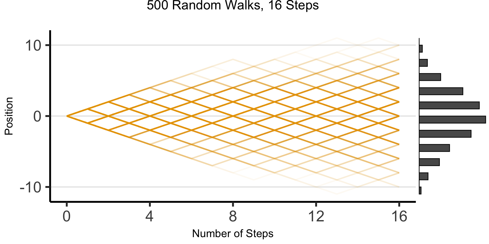
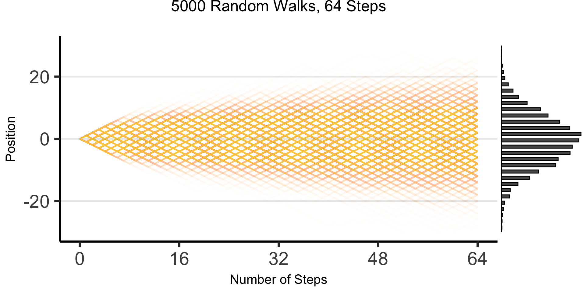
The Result: 64 Steps
“Mathematical/Scientific Modeling”
- Thing we observe (poking out of water): data
- Hidden but possibly discoverable through deeper investigation (ecosystem under surface): model / DGP

The Intuitive But Boring Problem of Causal Inference
library(dplyr)
library(ggplot2)
ga_lawyers <- c(21362, 22254, 23134, 23698, 24367, 24930, 25632, 26459, 27227, 27457)
ski_df <- tibble::tribble(
  ~year, ~varname, ~value,
  2000, "ski_revenue", 1551,
  2001, "ski_revenue", 1635,
  2002, "ski_revenue", 1801,
  2003, "ski_revenue", 1827,
  2004, "ski_revenue", 1956,
  2005, "ski_revenue", 1989,
  2006, "ski_revenue", 2178,
  2007, "ski_revenue", 2257,
  2008, "ski_revenue", 2476,
  2009, "ski_revenue", 2438,
)
ski_mean <- mean(ski_df$value)
ski_sd <- sd(ski_df$value)
ski_df <- ski_df %>% mutate(val_scaled = 12*value, val_norm = (value - ski_mean)/ski_sd)
law_df <- tibble::tibble(year=2000:2009, varname="ga_lawyers", value=ga_lawyers)
law_mean <- mean(law_df$value)
law_sd <- sd(law_df$value)
law_df <- law_df %>% mutate(val_norm = (value - law_mean)/law_sd)
spur_df <- dplyr::bind_rows(ski_df, law_df)
ggplot(spur_df, aes(x=year, y=val_norm, color=factor(varname, labels = c("Ski Revenue","Lawyers in Georgia")))) +
  stat_smooth(method="loess", se=FALSE) +
  geom_point(size=g_pointsize/1.5) +
  labs(
    fill="",
    title="Ski Revenue vs. Georgia Lawyers",
    x="Year",
    color="Correlation: 99.2%",
    linetype=NULL
  ) +
  theme_dsan() +
  scale_x_continuous(
    breaks=seq(from=2000, to=2014, by=2)
  ) +
  #scale_y_continuous(
  #  name="Total Revenue, Ski Facilities (Million USD)",
  #  sec.axis = sec_axis(~ . * law_sd + law_mean, name = "Number of Lawyers in Georgia")
  #) +
  scale_y_continuous(breaks = -1:1,
    labels = ~ . * round(ski_sd,1) + round(ski_mean,1),
    name="Total Revenue, Ski Facilities (Million USD)",
    sec.axis = sec_axis(~ . * law_sd + law_mean, name = "Number of Lawyers in Georgia")) +
  expand_limits(x=2010) +
  #geom_hline(aes(yintercept=x, color="Mean Values"), as.data.frame(list(x=0)), linewidth=0.75, alpha=1.0, show.legend = TRUE) +
  scale_color_manual(
    breaks=c('Ski Revenue', 'Lawyers in Georgia'),
    values=c('Ski Revenue'=cbPalette[1], 'Lawyers in Georgia'=cbPalette[2])
  )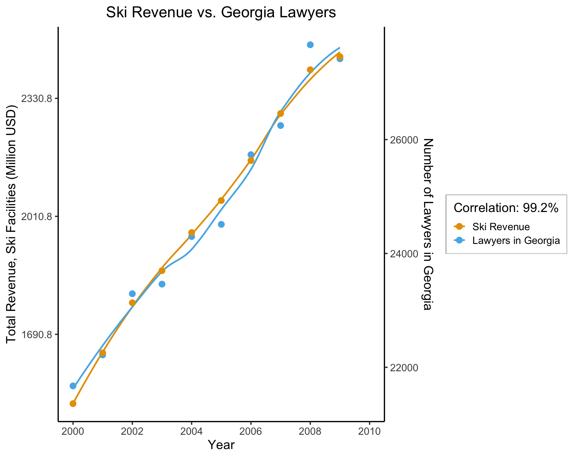
(Based on Spurious Correlations, Tyler Vigen)
- This, however, is only a mini-boss. Beyond it lies the truly invincible FINAL BOSS… 🙀
What Is To Be Done?
Selecting on the Dependent Variable
What “““research”“” “““says”“” about identifying people who might commit mass shootings
- Jeff’s ABHYSIOWDCI claim: If we care about intervening to reduce social ills, this literally has negative value (Goes up to zero value if you don’t publish it though! 😉)
(Annoying But Hopefully You’ll See the Importance Once We Digest Causal Inference… a standard term in The Sciences)
Chalkboard Time…
- \(\Pr(Y = 1) = \; ?\)
- \(\Pr(Y = 1 \mid E = 1) = \; ?\)

The Problem of Colliders
- \(X\) and \(Y\) are diseases which occur independently, no interrelationship, with probability \(1/3\)
- Either \(X\) or \(Y\) sufficient for admission to hospital, \(Z\)
- We have: \(X \rightarrow Z \leftarrow Y\) [🚨 Collider alert!]

What’s the Issue?
If we only have data on patients (\(Z = 1\)), observing \(X = 1\) lowers \(\Pr(Y = 1)\), despite the fact that \(X \perp Y\)!
\(X \perp Y\), but \((X \not\perp Y) \mid Z\)
The moral: controlling for stuff does not necessarily solve problem of causal inference, and can actually make it worse (inducing correlations where they don’t actually exist) 😭


The Final Diagrammatic Boss: SWIGs
- Single World Intervention Graphs


