Week 7: Markov Models

DSAN 5100: Probabilistic Modeling and Statistical Computing
Section 01

Class Sessions

Author

Purna Gamage, Amineh Zadbood, and Jeff Jacobs

Published

Tuesday, October 14, 2025

Motivation

source("../dsan-globals/_globals.r")

The Course So Far

Logic: Reasoning about T/F statements using and and or
$\rightarrow$ Set Theory: Reasoning about collections of objects and their union and intersection

Deterministic

Probabilistic

$\rightarrow$ Probability: Assigning “likelihood values” in $[0,1]$ to logical/set-theoretic statements about outcomes
$\rightarrow$ Random Variables: Doing math (beyond and and or) with the probabilities of these uncertain outcomes
All have been reasoning about uncertainty in more and more complex ways!

The New Dimension: Evolution Through Time

Markov models are a stepping-stone towards full-on time series analysis: reasoning about uncertainty over time
So why are time series the topic of an entire course, while Markov models only the topic of one week in DSAN5000?

Recall: Definition of Conditional Probability

\[ \Pr(A \mid B) \definedas \frac{\Pr(A, B)}{\Pr(B)} \genfrac{}{}{0pt}{}{\leftarrow A\text{ and }B\text{ happen}}{\leftarrow \text{In world where }\Omega = B} \]

The Markov Property

\[ P(\text{future} \mid \text{present}, {\color{orange}\text{past}}) = P(\text{future} \mid \text{present}) \]

The Markov Assumption

Often stated in many different (confusing) ways, but think of anterograde amnesia:

Keeping Track of States

Since Markov models come more from engineering than “pure” math/probability, we have “fancier” objects we’re keeping track of, rather than just Random Variables
We now keep track of the state of a system over time: this could be a single RV, but could be a collection of multiple (potentially dependent) RVs

What Information Should We Keep Track Of?

Sometimes answer seems “obvious”, lulls us into false sense of confidence (that we don’t have to think too hard about it)¹

System	State Space
Chess	Position of each piece, whose turn it is
Indoor Robot	Model of room + objects inside it
Predator-Prey Ecosystem	Relative species populations
Move Left/Move Right Game	?
Weather Prediction	?
Music	?

Tension between too little information (cannot model phenomena of interest) vs. too much information (solving model becomes intractable)

Modeling Music: Where is the Downbeat?

State Space Choice $\rightarrow$ Information Loss

Recall the Move Left/Move Right Game (especially from Lab 4 Prep)

Possible State Spaces:

History vector	Position	Steps	#L	#R
$()$	$x = 0$	0	0	0
$(L,R)$	$x = 0$	2	1	1
$(R,L)$	$x = 0$	2	1	1
$(R,L,R,$ $~L,R,L)$	$x = 0$	6	3	3
$(L)$	$x = -1$	1	1	0
$(L,L,R)$	$x = -1$	3	2	1

Markov Models

Finite-State Automata

(Deterministic!) Only “accepts” strings with even number of 1s:

Input String	Result	Input String	Result
$\varepsilon$	✅	`01`
`0`	✅	`10`
`1`		`1000000`
`00`	✅	`10000001`	✅

…But we’re trying to model probabilistic evolution!

Enter Markov Chains

Graphically

Mathematically

\[ \begin{array}{c c} & \begin{array}{c c c} 1 & 2 & 3 \\ \end{array} \\ \begin{array}{c c c}1 \\ 2 \\ 3 \end{array} & \left[ \begin{array}{c c c} 0 & 1/2 & 1/2 \\ 1/3 & 0 & 2/3 \\ 1/3 & 2/3 & 0 \end{array} \right] \end{array} \]

\[ \begin{array}{c c} & \begin{array}{c c c} 1 & 2 & 3 \\ \end{array} \\ \begin{array}{c c c}1 \\ 2 \\ 3 \end{array} & \left[ \begin{array}{c c c} 1/2 & 1/3 & 1/6 \\ 1/10 & 1/2 & 2/5 \\ 1/8 & 3/8 & 1/2 \end{array} \right] \end{array} \]

Hidden Markov Models

Use observed data to infer unobserved variables

(What our brains are doing, most of the time!)

PageRank

PageRank (Matrix Magic)

What is the relevance of this abstract topic? …🤑

library(readr)
library(ggplot2)
goog_df <- read_csv("assets/google_yearly_revenue.csv")
ggplot(goog_df, aes(x=year, y=revenue_billions)) +
  geom_bar(stat="identity", fill=cbPalette[1]) +
  labs(
    title = "Google Yearly Revenue, 2002-2022",
    x = "Year",
    y = "Revenue (Billion USD)"
  ) +
  dsan_theme("full")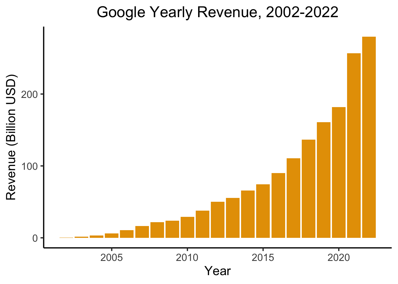

PageRank = The “spark” that ignited the Google flame

PageRank Visualized

Nodes = Webpages, Edges = Links

Goal: Rank the relative “importance” of a site $S_i$, taking into account the importance of other sites that link to $S_i$
- “Important” sites: linked to often, and linked to often by other important sites

Chickens and Eggs

Paradoxical at first: how are we supposed to figure out the importance of a site $S_i$, when that’s determined by
- the importance of sites $S_j$ that link to $S_i$, which is determined by
  - the importance of sites $S_k$ that link to sites $S_j$, which is determined by
    - the importance of the sites $S_\ell$ that link to those sites $S_k$, which is determined by…

\[ \begin{align*} \mathsf{Importance}(S_i) &= f(\mathsf{Importance}(S_{j \rightarrow i})) = f(f(\mathsf{Importance}(S_{k \rightarrow j \rightarrow i}))) \\ &= f(f(f(\mathsf{Importance}(S_{\ell \rightarrow k \rightarrow j \rightarrow i})))) = \cdots \end{align*} \]

Sanity hint: Remember infinite sums from calculus! They can converge, despite having infinitely-many terms… This is something like that, but for recursion (the mathematical term for an object whose definition refers to itself)

Resolving Recursive Definitions

We can compute this importance ranking, despite its recursive definition!
Recall, for example, the Fibonacci sequence: $1, 1, 2, 3, 5, 8, 13, 21, \ldots$
Defined recursively!

\[ f(n) = \begin{cases} 1 & n = 1\text{ or }n = 2 \\ f(n-2) + f(n-1) & n > 2 \end{cases} \]

And yet, a guy named Bernoulli figured out

\[ f(n) = \frac{\varphi^n - \psi^n}{\varphi - \psi} = \frac{\varphi^n - \psi^n}{\sqrt{5}}, \]

where $\varphi$ is the “Golden Ratio” $\frac{1 + \sqrt{5}}{2}$ and $\psi$ its conjugate $\frac{1 - \sqrt{5}}{2}$.

The PageRank Process

Every site starts with equal PageRank score: $r^{(0)}_1 = r^{(0)}_2 = r^{(0)}_3 = \frac{1}{3}$.
Each link $S_i \rightarrow S_j$ is a vote of confidence that $S_i$ is giving to $S_j$
At each time $t$, a site $S_i$ “spends” whatever voting power it currently has ($r^{(t)}_i$) on the sites it links to.
- $S_1$ casts one vote for itself and one vote for $S_2$, thus spending $\frac{1}{2}$ of its total PageRank on itself and $\frac{1}{2}$ of its total PageRank on $S_2$.
State of the process at time $t$: $\mathbf{r}^{(t)} = \begin{bmatrix}r^{(t)}_1 & r^{(t)}_2 & r^{(t)}_3\end{bmatrix}^\top$
Can form a matrix specifying how this state evolves from time $t$ to time $t+1$!

\[ \mathbf{E} = \begin{bmatrix} \frac{1}{2} & \frac{1}{2} & 0 \\ \frac{1}{2} & 0 & 1 \\ 0 & \frac{1}{2} & 0 \end{bmatrix} \; \leadsto \; \mathbf{r}^{(t+1)} = \mathbf{E}\mathbf{r}^{(t)} \]

Given the “$S_1$ casts one vote for itself…” part, can you say exactly what $S_1$ will “spend” on itself and on $S_2$ at time $t = 0$ (in the first round)?

We can use $\mathbf{E}$ to figure out the state at each step, starting from $t = 0$!

\[ \begin{array}{c@{}c@{}c@{}c@{}c@{}c@{}c} \mathbf{r}^{(1)} & = & \mathbf{E}\mathbf{r}^{(0)} & = & \begin{bmatrix} \frac{1}{2} & \frac{1}{2} & 0 \\ \frac{1}{2} & 0 & 1 \\ 0 & \frac{1}{2} & 0 \end{bmatrix}\begin{bmatrix} \frac{1}{3} \\ \frac{1}{3} \\ \frac{1}{3}\end{bmatrix} & = & \begin{bmatrix} \frac{1}{3} \\ \frac{1}{2} \\ \frac{1}{6} \end{bmatrix} \\ ~ & ~ & ~ & ~ & ~ & \swarrow & ~ \\ \mathbf{r}^{(2)} & = & \mathbf{E}\mathbf{r}^{(1)} & = & \begin{bmatrix} \frac{1}{2} & \frac{1}{2} & 0 \\ \frac{1}{2} & 0 & 1 \\ 0 & \frac{1}{2} & 0 \end{bmatrix}\begin{bmatrix}\frac{1}{3} \\ \frac{1}{2} \\ \frac{1}{6}\end{bmatrix} & = & \begin{bmatrix}\frac{5}{12} \\ \frac{1}{3} \\ \frac{1}{4}\end{bmatrix} \\ ~ & ~ & ~ & ~ & ~ & \swarrow & ~ \\ \mathbf{r}^{(3)} & = & \mathbf{E}\mathbf{r}^{(2)} & = & \cdots & ~ & ~ \end{array} \]

Matrix Magic

(1) Won’t we just have to run this forever? (2) How do we know it’ll converge to something?
Answers: (1) No! (2) because Markov matrix magic!
“Steady state” = state where $\mathbf{r}^{(t)} = \mathbf{r}^{(t+1)} = \mathbf{r}^{(t+2)} = \cdots \definedas \mathbf{r}^*$. But this means

\[ \mathbf{r}^{(t+1)} = \mathbf{r}^{(t)} \iff \mathbf{E}\mathbf{r}^{(t)} = \mathbf{r}^{(t)} \iff \mathbf{E}\mathbf{r}^* = \mathbf{r}^* \]

This $\mathbf{r}^*$ is (by definition!) an Eigenvector of $\mathbf{E}$ with Eigenvalue $\lambda = 1$!²

In my opinion, along with e.g. insolubility of the quintic, this is maybe the most mind-blowing case of math magic :3

Solving the Matrix Magic

Since we already know the Eigenvalue of interest, $\lambda = 1$, all that’s left is solving for its corresponding Eigenvector:

\[ \mathbf{E}\mathbf{r}^* = \mathbf{r}^* \iff \mathbf{E}\mathbf{r}^* - \mathbf{r}^* = \mathbf{0} \iff (\mathbf{E} - \mathbf{I})\mathbf{r}^* = \mathbf{0} \]
Written out, we see that this gives us a system of linear equations:

\[ \begin{bmatrix} \frac{1}{2} & \frac{1}{2} & 0 \\ \frac{1}{2} & 0 & 1 \\ 0 & \frac{1}{2} & 0 \end{bmatrix}\begin{bmatrix}r^*_1 \\ r^*_2 \\ r^*_3\end{bmatrix} = \begin{bmatrix}0 \\ 0 \\ 0\end{bmatrix} \iff \begin{array}{ccccccc}\frac{1}{2}r^*_1 & + & \frac{1}{2}r^*_2 & ~ & ~ & = & 0 \\ \frac{1}{2}r^*_1 & ~ & ~ & + & r^*_3 & = & 0 \\ ~ & ~ & \frac{1}{2}r^*_2 & ~ & ~ & = & 0\end{array} \]

which we can solve however we want!
To handle the fact that this system is underspecified, impose additional restriction that $r^*_1 + r^*_2 + r^*_3 = 1$, so that the ranks form a probability distribution

The Point of All This

The final restriction $r^*_1 + r^*_2 + r^*_3 = 1$ ensures that the resulting PageRank values form a probability distribution
This is called the Stationary Distribution of the Markov chain: represents the probability that a random walker through the chain will be at page $S_i$ at a given time!
- Equivalently: expected proportion of total walking time a random-walker will spend at each node
Every Markov chain has a Stationary Distribution! This fact has cool implications even above and beyond the Google $$$ implications 😜

Footnotes

To snap out of this lull, keep in mind that engineering/nonlinear dynamical systems programs have entire courses just on state space representations↩︎
This is because an Eigenvalue-Eigenvector pair for a matrix $\mathbf{M}$ is a vector $\mathbf{v}$ and scalar value $\lambda$ which satisfy $\mathbf{M}\mathbf{v} = \lambda \mathbf{v}$. In words: the result of (left) matrix-multiplying $\mathbf{v}$ by $\mathbf{M}$ is the same as scalar-multiplying $\mathbf{v}$ by a factor of $\lambda$. In our case the Eigenvector is $\mathbf{r}^*$ and the Eigenvalue is $\lambda = 1$, since $\mathbf{E}\mathbf{r}^* = 1 \cdot \mathbf{r}^*$.
For the math-curious, there are lots of fun results from matrix theory which assure us that $\mathbf{E}$ is guaranteed to have principal eigenvalue $\lambda = 1$ 💆↩︎

History vector	Position	Steps	#L	#R
\(()\)	\(x = 0\)	0	0	0
\((L,R)\)	\(x = 0\)	2	1	1
\((R,L)\)	\(x = 0\)	2	1	1
\((R,L,R,\) \(~L,R,L)\)	\(x = 0\)	6	3	3
\((L)\)	\(x = -1\)	1	1	0
\((L,L,R)\)	\(x = -1\)	3	2	1