Week 6: Multivariate Distributions

DSAN 5100: Probabilistic Modeling and Statistical Computing
Section 01

Class Sessions

Author

Purna Gamage, Amineh Zadbood, and Jeff Jacobs

Published

Tuesday, September 30, 2025

Distributions in Continuous World

source("../dsan-globals/_globals.r")

Discrete = “Easy mode”: Based (intuitively) on sets
\(\Pr(A)\): Four equally-likely marbles \(\{A, B, C, D\}\) in box, what is probability I pull out \(A\)?

library(tibble)
library(ggplot2)
disc_df <- tribble(
  ~x, ~y, ~label,
  0, 0, "A",
  0, 1, "B",
  1, 0, "C",
  1, 1, "D"
)
disc_df |> ggplot(aes(x=x, y=y, label=label)) +
  geom_point(size=g_pointsize) +
  geom_text(
    size=g_textsize,
    hjust=1.5,
    vjust=-0.5
  ) +
  xlim(-0.5,1.5) + ylim(-0.5,1.5) +
  coord_fixed() +
  dsan_theme("quarter") +
  theme(
    panel.background = element_rect(
      fill = "transparent",
      color = NA_character_
    ),
    plot.background = element_rect(
      fill = "transparent",
      color = NA_character_
    ),
    rect = element_rect(fill = "transparent"),
  ) +
  labs(title="Discrete Probability Space")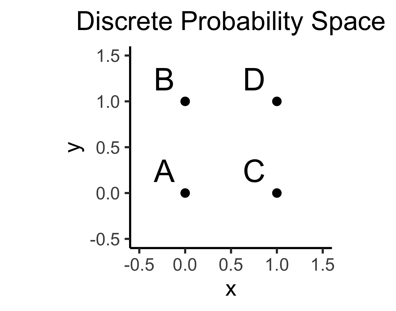

\[ \Pr(A) = \underset{\mathclap{\small \text{Probability }\textbf{mass}}}{\boxed{\frac{|\{A\}|}{|\Omega|}}} = \frac{1}{|\{A,B,C,D\}|} = \frac{1}{4} \]

Continuous = “Hard mode”: Based (intuitively) on areas
\(\Pr(A)\): Throw dart at random point in square, what is probability I hit \(\require{enclose}\enclose{circle}{\textsf{A}}\)?

library(ggforce)
disc_df |> ggplot(aes(x=x, y=y, label=label)) +
  xlim(-0.5,1.5) + ylim(-0.5,1.5) +
  geom_rect(aes(xmin = -0.5, xmax = 1.5, ymin = -0.5, ymax = 1.5), fill=cbPalette[1], color="black", alpha=0.3) +
  geom_circle(aes(x0=x, y0=y, r=0.25), fill=cbPalette[2]) +
  coord_fixed() +
  dsan_theme("quarter") +
  geom_text(
    size=g_textsize,
    #hjust=1.75,
    #vjust=-0.75
  ) +
  geom_text(
    data=data.frame(label="Ω"),
    aes(x=-0.4,y=1.39),
    parse=TRUE,
    size=10
  ) +
  theme(
    panel.background = element_rect(
      fill = "transparent",
      color = NA_character_
    ),
    plot.background = element_rect(
      fill = "transparent",
      color = NA_character_
    ),
    rect = element_rect(fill = "transparent"),
  ) +
  labs(title="Continuous Probability Space")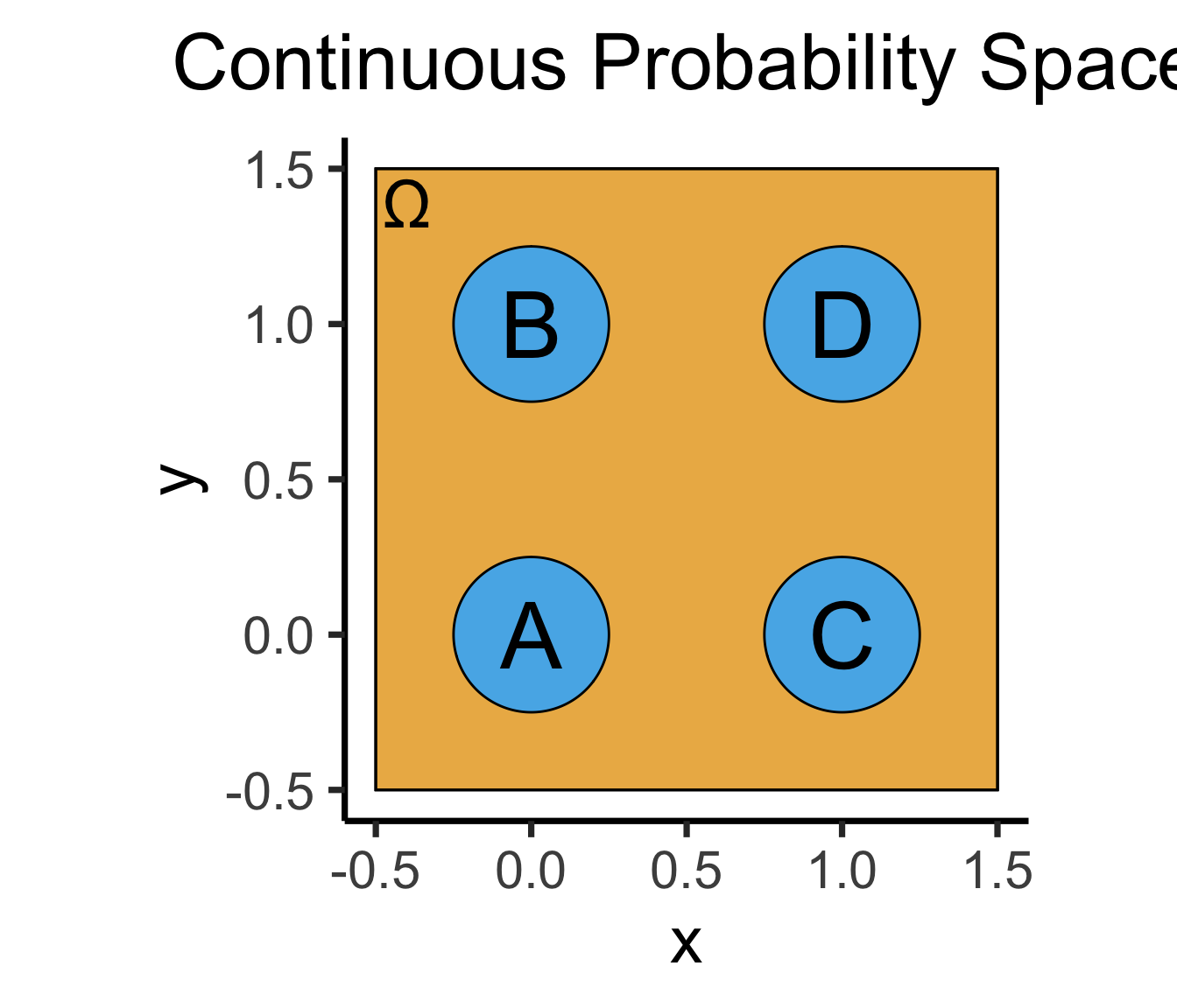

\[ \Pr(A) = \underset{\mathclap{\small \text{Probability }\textbf{density}}}{\boxed{\frac{\text{Area}(\{A\})}{\text{Area}(\Omega)}}} = \frac{\pi r^2}{s^2} = \frac{\pi \left(\frac{1}{4}\right)^2}{4} = \frac{\pi}{64} \]

Moving to Continuous World

Intuitions from discrete world do translate into good intuitions for continuous world, in this case!
Can “move” discrete table into continuous space like Riemann sums “move” discrete sums into integrals:

“Smoothing” Our Example

Instead of discrete \(G\) with \(\mathcal{R}_G = \{10, 11, 12\}\), we have continuous \(G\) with \(\mathcal{R}_G = [10,12] \subset \mathbb{R}\) (HS progress)
Instead of discrete \(H\) with \(\mathcal{R}_H = \{0, 1\}\), now we keep track of continuous “honors spectrum” \(H\) with \(\mathcal{R}_H = [0, 1] \subset \mathbb{R}\)
Student near beginning of 10th grade who is at “high end” of honors spectrum: \(G = 10.03\) and \(H = 0.95\)

“Smoothing” Our Tables

	Discrete World	Continuous World
How do we get probabilities?	Sums \(\Pr(X = 1)\) \(+ \Pr(X = 2) = \frac{2}{6}\)	Integrals \(\displaystyle\int_{x=20}^{x=21}f_X(x) = 0.4\)
What makes a valid distribution?	\(\displaystyle\sum_{x \in \mathcal{R}_X}\Pr(X = x) = 1\)	\(\displaystyle\int_{x \in \mathcal{R}_X}f_X(x) = 1\)
How do we model uncertainty about multiple variables?	Frequency table	Joint pdf

Continuous Joint pdfs

The volume of this Hershey Kiss is exactly \(1\)
Integrating over a region \(C\) gives us

\[ \frac{\text{Volume}(\{(X,Y) \mid (X,Y) \in C\})}{\text{Volume}(\text{Hershey Kiss})} = \Pr((X,Y) \in C) \]

Figure 3.11 from DeGroot and Schervish (2013)

Conditional pdfs

Now, if we learn that \(Y = y_0\), can take “slice” at \(y = y_0\)
Total area of this slice is not \(1\), so \(f_{X,Y}(x, y_0)\) is not a valid pdf
Dividing by total area of slice would generate valid pdf. What is this area? \(f_X(y_0)\)
\(\implies\) \(f_{X \mid Y = y_0}(x \mid y_0) = \frac{f_{X,Y}(x, y_0)}{f_X(y_0)}\) is valid (conditional) pdf

Figure 3.20 from DeGroot and Schervish (2013)

Working Backwards in Continuous World

While in discrete world we could easily provide a table, in continuous world we often/usually have to work backwards; we may just be given:
\(G \sim \mathcal{U}(10, 12)\)
\(H \sim \ddot{\mathcal{N}}(\mu = 0.5, \sigma = 0.1, a = 0, b = 1)\), and
\(G \perp H\) (so \(\Pr(G \mid H) = \Pr(G), \Pr(H \mid G) = \Pr(H)\))
(i.e., marginal distributions = conditional distributions)

The Marginal pdfs of \(G\) and \(H\)

Since we know \(G \sim \mathcal{U}(10,12)\), we know (or we could look up) that \(G\) has pdf

\[ f_G(g) = \frac{1}{12 - 10} = \frac{1}{2} \]

\(H\) has a slightly fancier distribution: truncated normal
Nonetheless a pdf we can derive from (a) knowing the pdf of the normal distribution and (b) knowing what we’ve just talked about regarding conditional distributions

The Truncated Normal Distribution

\(\ddot{\mathcal{N}}\) may look scary, but \(X \sim \ddot{\mathcal{N}}(\mu, \sigma, a, b)\) just means \(X\) can be constructed as:

\[ X \sim \mathcal{N}(\mu, \sigma) \leadsto [X \mid a < X < b] \sim \ddot{\mathcal{N}}(\mu, \sigma, a, b) \]

rnormt <- function(n, range, mu, s = 1) {
  
  # range is a vector of two values
  
  F.a <- pnorm(min(range), mean = mu, sd = s)
  F.b <- pnorm(max(range), mean = mu, sd = s)
  
  u <- runif(n, min = F.a, max = F.b)
  
  qnorm(u, mean = mu, sd = s)
  
}
library(data.table)
library(simstudy)
library(paletteer)
defC <- defCondition(condition= "tt == 1", 
                     formula = "rnormt(10000, c(-Inf, Inf), mu = 0, s = 3)")
defC <- defCondition(defC, "tt == 2", 
                     formula = "rnormt(10000, c(0, Inf), mu = 0, s = 3)")
defC <- defCondition(defC, "tt == 3", 
                     formula = "rnormt(10000, c(-3, 3.5), mu = 0, s = 3)")

dd <- genData(30000)
dd <- trtAssign(dd, nTrt = 3, grpName = "tt")
dd <- addCondition(defC, dd, "x")
dd[, tt := factor(tt, 
     labels = c("No truncation", "Left truncation at 0", "Left and right truncation"))]
dd |> ggplot(aes(x = x, group = tt)) +
  geom_histogram(
    aes(fill = tt, y=after_stat(density)),
    alpha = 1, binwidth = .2, boundary = 0
  ) +
  facet_grid(~tt) +
  theme(
    panel.grid = element_blank(),
    axis.title = element_blank(),
  ) +
  dsan_theme() +
  remove_legend()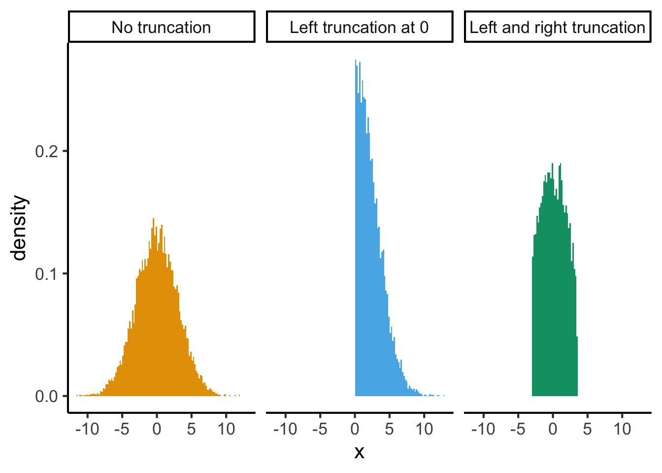

Adapted from `simstudy` package documentation

The Truncated Normal pdf

Since we see a conditioning bar on the previous slide, we can infer what the pdf of this conditional distribution would look like. If \(X \sim \ddot{\mathcal{N}}(\mu, \sigma, a, b)\), then \(X\) has pdf

\[ f_X(x) = \frac{1}{\sigma}\cdot \frac{\varphi\left(\frac{x - \mu}{\sigma}\right)}{\Phi\left(\frac{b-\mu}{\sigma}\right) - \Phi\left(\frac{a - \mu}{\sigma}\right)} \approx \frac{\Pr(X \approx x, a < X < b)}{\Pr(a < X < b)} \]

\(\varphi\) is the pdf of \(\mathcal{N}(0,1)\)
\(\Phi\) is the CDF of \(\mathcal{N}(0,1)\)

(Note the lowercasing to describe pdfs and capitalizing to describe CDFs, even in Greek!)

Back to Working Backwards

By definition of independence, we can obtain joint pdf \(f_{G,H}(g, h)\) by multiplying marginal pdf \(f_G(g)\) and marginal pdf \(f_H(h)\):

\[ \begin{align*} f_{G,H}(g, h) &= f_G(g) \cdot f_H(h) \\ &= \frac{1}{2} \cdot \left[ \frac{1}{0.1} \cdot \frac { \varphi\left(\frac{h - 0.5}{0.1}\right) } { \Phi\left(\frac{12-0.5}{0.1}\right) - \Phi\left(\frac{10 - 0.5}{0.1}\right) } \right] \end{align*} \]

Moving Forwards Again

We’ve arrived at the case we had in discrete world, where we know the joint distribution!
We can integrate wherever we took sums in the discrete case to obtain marginal pdfs:

\[ \begin{align*} f_G(g) &= \int_{0}^{1}f_{G,H}(g,h)\mathrm{d}h = \frac{1}{2}, \\ f_H(h) &= \int_{10}^{12}f_{G,H}(g, h)\mathrm{d}g = \frac{1}{0.1} \cdot \frac { \varphi\left(\frac{h - 0.5}{0.1}\right) } { \Phi\left(\frac{12 - 0.5}{0.1}\right) - \Phi\left(\frac{10 - 0.5}{0.1}\right) } \end{align*} \]

Conditional Distributions in Continuous World

We can compute conditional pdfs by renormalizing
Denominator is no longer integral of the distribution over all possible values (hence just the number \(1\)), but a ratio of joint distribution to marginal distribution values like:

\[ f_{H \mid G}(h | g) = \frac{f_{G,H}(g, h)}{f_G(g)}. \]

At first this is magic… we can use the exact same equation from discrete world?!?
But then you remember, continuous world was set up as a “hack”, using area under the curve between two points rather than height of the curve at a point to “port” discrete formulas into continuous world
Think of how, when mathematicians hit the “wall” of solving \(x^2 + 1 = 0\)… They set up a new number \(i\) to work with these polynomials using “standard” algebra. Here we set up continuous pdf \(f_X(x)\) to work with continuous RVs using “standard” probability theory!

You Don’t Have To Stare Helplessly At Scary Math!

Try to link the continuous equations back to their simpler discrete forms
Work with the discrete forms to develop intuition, then
Convert sums back into integrals once you’re ready

A Concrete Strategy

Start by discretizing (“binning”) the possible values of a continuous RV to obtain a discrete RV:
- Split \([10,12]\) into three equal-length bins, \([0,1]\) into two equal-length bins
- Simulate \((G, H)\) pairs, sort into bins, plot joint / marginal / conditional distributions of binned data
As you make bins thinner and thinner… 🤔

Thinking Through Specific Multivariate Distributions

From \(2\) to \(N\) variables!

The Multinoulli Distribution

May seem like a weird/contrived distribution, but is perfect for building intuition, as your first \(N\)-dimensional distribution (\(N > 2\))
\(\mathbf{X}\) is a six-dimensional Vector-Valued RV, so that

\[ \mathbf{X} = (X_1, X_2, X_3, X_4, X_5, X_6), \]

where \(\mathcal{R}_{X_1} = \{0, 1\}, \mathcal{R}_{X_2} = \{0, 1\}, \ldots, \mathcal{R}_{X_6} = \{0, 1\}\)
But, \(X_1, X_2, \ldots, X_6\) are not independent! In fact, they are so dependent that if one has value \(1\), the rest must have value \(0\) \(\leadsto\) we can infer the support of \(\mathbf{X}\):

\[ \begin{align*} \mathcal{R}_{\mathbf{X}} = \{ &(1,0,0,0,0,0),(0,1,0,0,0,0),(0,0,1,0,0,0), \\ &(0,0,0,1,0,0),(0,0,0,0,1,0),(0,0,0,0,0,1)\} \end{align*} \]
Lastly, need to define the probability that \(\mathbf{X}\) takes on any of these values. Let’s say \(\Pr(\mathbf{X} = \mathbf{v}) = \frac{1}{6}\) for all \(\mathbf{v} \in \mathcal{R}_{\mathbf{X}}\). Do we see the structure behind this contrived case?
(For math major friends, there is an isomorphism afoot… For the rest, it’s an extremely inefficient way to model outcomes from rolling a fair die)

The Multivariate Normal Distribution

We’ve already seen the matrix notation for writing the parameters of this distribution: \(\mathbf{X}_{[k \times 1]} \sim \mathcal{N}_k\left(\boldsymbol\mu_{[k \times 1]}, \Sigma_{[k \times k]}\right)\)
Now we get to crack open the matrix notation for writing its pdf:

\[ f_\mathbf{X}(\mathbf{x}_{[k \times 1]}) = \underbrace{\left(\frac{1}{\sqrt{2\pi}}\right)^k \frac{1}{\sqrt{\det(\Sigma)}}}_{\text{Normalizing constants}} \exp\left(-\frac{1}{2}\underbrace{(\mathbf{x} - \boldsymbol\mu)^\top \Sigma^{-1} (\mathbf{x} - \boldsymbol\mu)}_{\text{Quadratic form}}\right) \]

Try to squint your eyes while looking at the above and compare with…

pdf of \(\mathcal{N}(\mu,\sigma)\)

\[ f_X(v) = \frac{1}{\sigma\sqrt{2\pi}}\bigexp{-\frac{1}{2}\left(\frac{v - \mu}{\sigma}\right)^2} \]

Structure of \(\Sigma\)

\[ \begin{align*} \mathbf{\Sigma} &= \begin{bmatrix}\sigma_1^2 & \rho\sigma_1\sigma_2 \\ \rho\sigma_2\sigma_1 & \sigma_2^2\end{bmatrix} \\[0.1em] \implies \det(\Sigma) &= \sigma_1^2\sigma_2^2 - \rho^2\sigma_1^2\sigma_2^2 \\ &= \sigma_1^2\sigma_2^2(1-\rho^2) \end{align*} \]

Quadratic Forms

Quadratic forms will seem scary until someone forces you to write out the matrix multiplication!
Start with the 1D case: \(\mathbf{x} = [x_1]\), \(\boldsymbol\mu = [\mu_1]\), \(\Sigma = [\sigma^2]\). Then

\[ (\mathbf{x} - \boldsymbol\mu)^\top \Sigma^{-1} (\mathbf{x - \boldsymbol\mu}) = (x_1 - \mu_1)\frac{1}{\sigma^2}(x_1 - \mu_1) = \left(\frac{x_1 - \mu_1}{\sigma}\right)^2 ~ 🤯 \]

The 2D Case

Let \(\mathbf{x} = \left[\begin{smallmatrix}x_1 \\ x_2\end{smallmatrix}\right]\), \(\boldsymbol\mu = \left[ \begin{smallmatrix}\mu_1 \\ \mu_2 \end{smallmatrix}\right]\), \(\Sigma\) as in previous slide. Then \(\mathbf{x} - \boldsymbol\mu = \left[ \begin{smallmatrix} x_1 - \mu_1 \\ x_2 - \mu_2 \end{smallmatrix} \right]\)
Using what we know about \(2 \times 2\) matrix inversion,

\[ \Sigma^{-1} = \frac{1}{\det(\Sigma)}\left[ \begin{smallmatrix} \sigma_2^2 & -\rho \sigma_2\sigma_1 \\ -\rho \sigma_1\sigma_2 & \sigma_1^2\end{smallmatrix} \right] = \frac{1}{\sigma_1^2\sigma_2^2(1-\rho^2)}\left[ \begin{smallmatrix} \sigma_2^2 & -\rho \sigma_2\sigma_1 \\ -\rho \sigma_1\sigma_2 & \sigma_1^2\end{smallmatrix} \right] \]

With \(\widetilde{\rho} \equiv 1 - \rho^2\), we can write everything as a bunch of matrix multiplications:

\[ \begin{align*} &(\mathbf{x} - \boldsymbol\mu)^\top \Sigma^{-1} (\mathbf{x} - \boldsymbol\mu) = \frac{1}{\sigma_1^2\sigma_2^2 \widetilde{\rho}} \begin{bmatrix}x_1 - \mu_1 & x_2 - \mu_2\end{bmatrix} \cdot \begin{bmatrix} \sigma_2^2 & -\rho \sigma_2\sigma_1 \\ -\rho \sigma_1\sigma_2 & \sigma_1^2\end{bmatrix} \cdot \begin{bmatrix}x_1 - \mu_1 \\ x_2 - \mu_2\end{bmatrix} \\ &= \frac{1}{\sigma_1^2\sigma_2^2 \widetilde{\rho}} \begin{bmatrix}(x_1-\mu_1)\sigma_2^2 - (x_2-\mu_2)\rho\sigma_1\sigma_2 & (x_2 - \mu_2)\sigma_1^2 - (x_1 - \mu_1)\rho\sigma_2\sigma_1 \end{bmatrix} \cdot \begin{bmatrix}x_1 - \mu_1 \\ x_2 - \mu_2\end{bmatrix} \\ &= \frac{1}{\sigma_1^2\sigma_2^2 \widetilde{\rho}} \left( (x_1-\mu_1)^2 \sigma_2^2 - (x_1 - \mu_1)(x_1 - \mu_2)\sigma_1\sigma_2 + (x_2 - \mu_2)^2 \sigma_1^2 - (x_1 - \mu_1)(x_2 - \mu_2)\sigma_2\sigma_1 \right) \\ &= \boxed{ \frac{1}{\widetilde{\rho}} \left( \left(\frac{x_1 - \mu_1}{\sigma_1}\right)^2 + \left(\frac{x_2 - \mu_2}{\sigma_2}\right)^2 - 2\rho\frac{(x_1 - \mu_1)(x_2 - \mu_2)}{\sigma_1\sigma_2} \right) } \end{align*} \]

The 2D Case In Its FINAL FORM

\[ f_{\mathbf{X}}(\mathbf{x}) = C \bigexp{ -\frac{1}{2(1-\rho^2)} \left( \left(\frac{x_1 - \mu_1}{\sigma_1}\right)^2 + \left(\frac{x_2 - \mu_2}{\sigma_2}\right)^2 - 2\rho\frac{(x_1 - \mu_1)(x_2 - \mu_2)}{\sigma_1\sigma_2} \right) } \]

where

\[ C = \frac{1}{2\pi\sigma_1\sigma_2\sqrt{1-\rho^2}}. \]

References

DeGroot, Morris H., and Mark J. Schervish. 2013. Probability and Statistics. Pearson Education.