Week 6: Multivariate Distributions

DSAN 5100: Probabilistic Modeling and Statistical Computing
Section 01

Purna Gamage, Amineh Zadbood, and Jeff Jacobs

Tuesday, September 30, 2025

Distributions in Continuous World

\[ \DeclareMathOperator*{\argmax}{argmax} \DeclareMathOperator*{\argmin}{argmin} \newcommand{\bigexp}[1]{\exp\mkern-4mu\left[ #1 \right]} \newcommand{\bigexpect}[1]{\mathbb{E}\mkern-4mu \left[ #1 \right]} \newcommand{\convergesAS}{\overset{\text{a.s.}}{\longrightarrow}} \newcommand{\definedas}{\overset{\text{def}}{=}} \newcommand{\definedalign}{\overset{\phantom{\text{def}}}{=}} \newcommand{\eqeventual}{\overset{\mathclap{\text{\small{eventually}}}}{=}} \newcommand{\Err}{\text{Err}} \newcommand{\expect}[1]{\mathbb{E}[#1]} \newcommand{\expectsq}[1]{\mathbb{E}^2[#1]} \newcommand{\fw}[1]{\texttt{#1}} \newcommand{\given}{\mid} \newcommand{\green}[1]{\color{green}{#1}} \newcommand{\heads}{\outcome{heads}} \newcommand{\iid}{\overset{\text{\small{iid}}}{\sim}} \newcommand{\lik}{\mathcal{L}} \newcommand{\loglik}{\ell} \newcommand{\mle}{\textsf{ML}} \newcommand{\nimplies}{\;\not\!\!\!\!\implies} \newcommand{\orange}[1]{\color{orange}{#1}} \newcommand{\outcome}[1]{\textsf{#1}} \newcommand{\param}[1]{{\color{purple} #1}} \newcommand{\pgsamplespace}{\{\green{1},\green{2},\green{3},\purp{4},\purp{5},\purp{6}\}} \newcommand{\prob}[1]{P\left( #1 \right)} \newcommand{\purp}[1]{\color{purple}{#1}} \newcommand{\sign}{\text{Sign}} \newcommand{\spacecap}{\; \cap \;} \newcommand{\spacewedge}{\; \wedge \;} \newcommand{\tails}{\outcome{tails}} \newcommand{\Var}[1]{\text{Var}[#1]} \newcommand{\bigVar}[1]{\text{Var}\mkern-4mu \left[ #1 \right]} \]

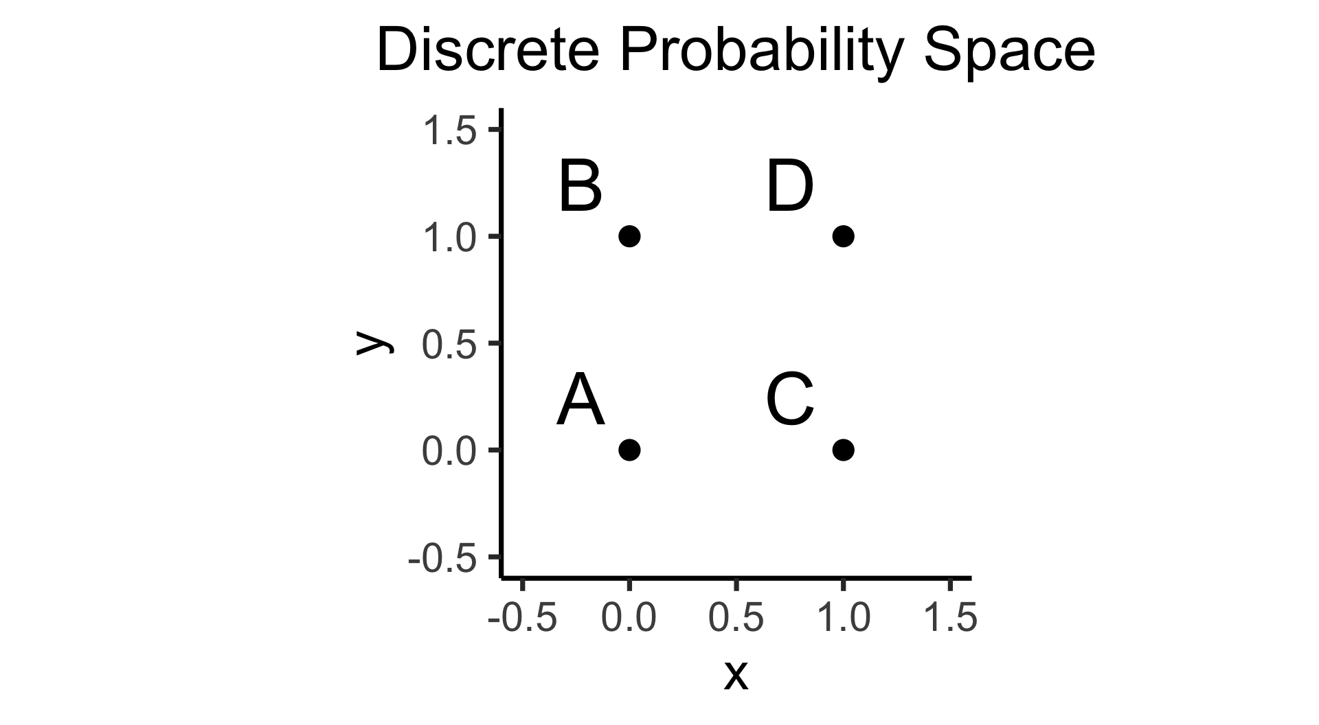
• Discrete = “Easy mode”: Based (intuitively) on sets
• \(\Pr(A)\): Four equally-likely marbles \(\{A, B, C, D\}\) in box, what is probability I pull out \(A\)?

\[ \Pr(A) = \underset{\mathclap{\small \text{Probability }\textbf{mass}}}{\boxed{\frac{|\{A\}|}{|\Omega|}}} = \frac{1}{|\{A,B,C,D\}|} = \frac{1}{4} \]

• Continuous = “Hard mode”: Based (intuitively) on areas
• \(\Pr(A)\): Throw dart at random point in square, what is probability I hit \(\require{enclose}\enclose{circle}{\textsf{A}}\)?

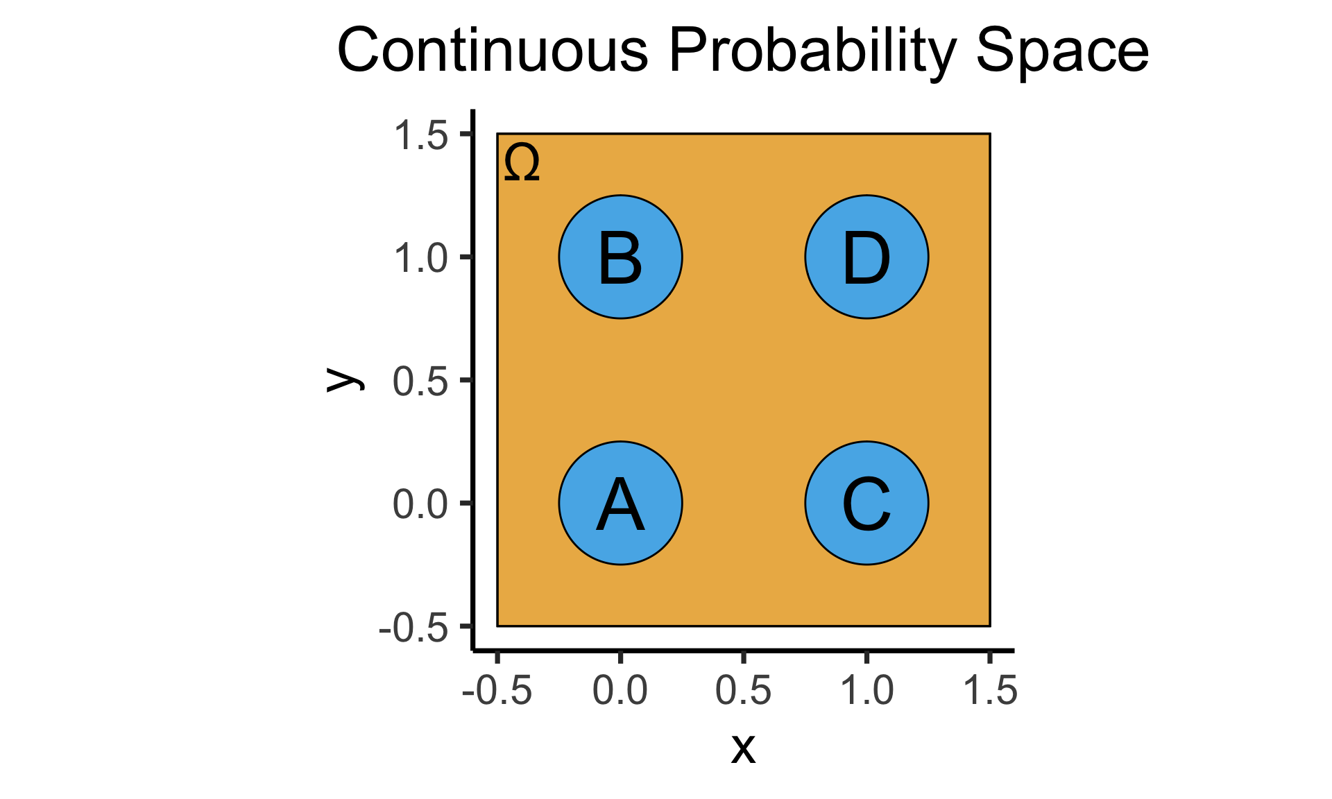
\[ \Pr(A) = \underset{\mathclap{\small \text{Probability }\textbf{density}}}{\boxed{\frac{\text{Area}(\{A\})}{\text{Area}(\Omega)}}} = \frac{\pi r^2}{s^2} = \frac{\pi \left(\frac{1}{4}\right)^2}{4} = \frac{\pi}{64} \]

Moving to Continuous World

• Intuitions from discrete world do translate into good intuitions for continuous world, in this case!
• Can “move” discrete table into continuous space like Riemann sums “move” discrete sums into integrals:

“Smoothing” Our Example

• Instead of discrete \(G\) with \(\mathcal{R}_G = \{10, 11, 12\}\), we have continuous \(G\) with \(\mathcal{R}_G = [10,12] \subset \mathbb{R}\) (HS progress)
• Instead of discrete \(H\) with \(\mathcal{R}_H = \{0, 1\}\), now we keep track of continuous “honors spectrum” \(H\) with \(\mathcal{R}_H = [0, 1] \subset \mathbb{R}\)
• Student near beginning of 10th grade who is at “high end” of honors spectrum: \(G = 10.03\) and \(H = 0.95\)

“Smoothing” Our Tables

	Discrete World	Continuous World
How do we get probabilities?	Sums \(\Pr(X = 1)\) \(+ \Pr(X = 2) = \frac{2}{6}\)	Integrals \(\displaystyle\int_{x=20}^{x=21}f_X(x) = 0.4\)
What makes a valid distribution?	\(\displaystyle\sum_{x \in \mathcal{R}_X}\Pr(X = x) = 1\)	\(\displaystyle\int_{x \in \mathcal{R}_X}f_X(x) = 1\)
How do we model uncertainty about multiple variables?	Frequency table	Joint pdf

Continuous Joint pdfs

• The volume of this Hershey Kiss is exactly \(1\)
• Integrating over a region \(C\) gives us

\[ \frac{\text{Volume}(\{(X,Y) \mid (X,Y) \in C\})}{\text{Volume}(\text{Hershey Kiss})} = \Pr((X,Y) \in C) \]

Figure 3.11 from DeGroot and Schervish (2013)

Conditional pdfs

• Now, if we learn that \(Y = y_0\), can take “slice” at \(y = y_0\)
• Total area of this slice is not \(1\), so \(f_{X,Y}(x, y_0)\) is not a valid pdf
• Dividing by total area of slice would generate valid pdf. What is this area? \(f_X(y_0)\)
• \(\implies\) \(f_{X \mid Y = y_0}(x \mid y_0) = \frac{f_{X,Y}(x, y_0)}{f_X(y_0)}\) is valid (conditional) pdf

Figure 3.20 from DeGroot and Schervish (2013)

Working Backwards in Continuous World

• While in discrete world we could easily provide a table, in continuous world we often/usually have to work backwards; we may just be given:
• \(G \sim \mathcal{U}(10, 12)\)
• \(H \sim \ddot{\mathcal{N}}(\mu = 0.5, \sigma = 0.1, a = 0, b = 1)\), and
• \(G \perp H\) (so \(\Pr(G \mid H) = \Pr(G), \Pr(H \mid G) = \Pr(H)\))
• (i.e., marginal distributions = conditional distributions)

The Marginal pdfs of \(G\) and \(H\)

• Since we know \(G \sim \mathcal{U}(10,12)\), we know (or we could look up) that \(G\) has pdf

\[ f_G(g) = \frac{1}{12 - 10} = \frac{1}{2} \]

• \(H\) has a slightly fancier distribution: truncated normal
• Nonetheless a pdf we can derive from (a) knowing the pdf of the normal distribution and (b) knowing what we’ve just talked about regarding conditional distributions

The Truncated Normal Distribution

• \(\ddot{\mathcal{N}}\) may look scary, but \(X \sim \ddot{\mathcal{N}}(\mu, \sigma, a, b)\) just means \(X\) can be constructed as:

\[ X \sim \mathcal{N}(\mu, \sigma) \leadsto [X \mid a < X < b] \sim \ddot{\mathcal{N}}(\mu, \sigma, a, b) \]

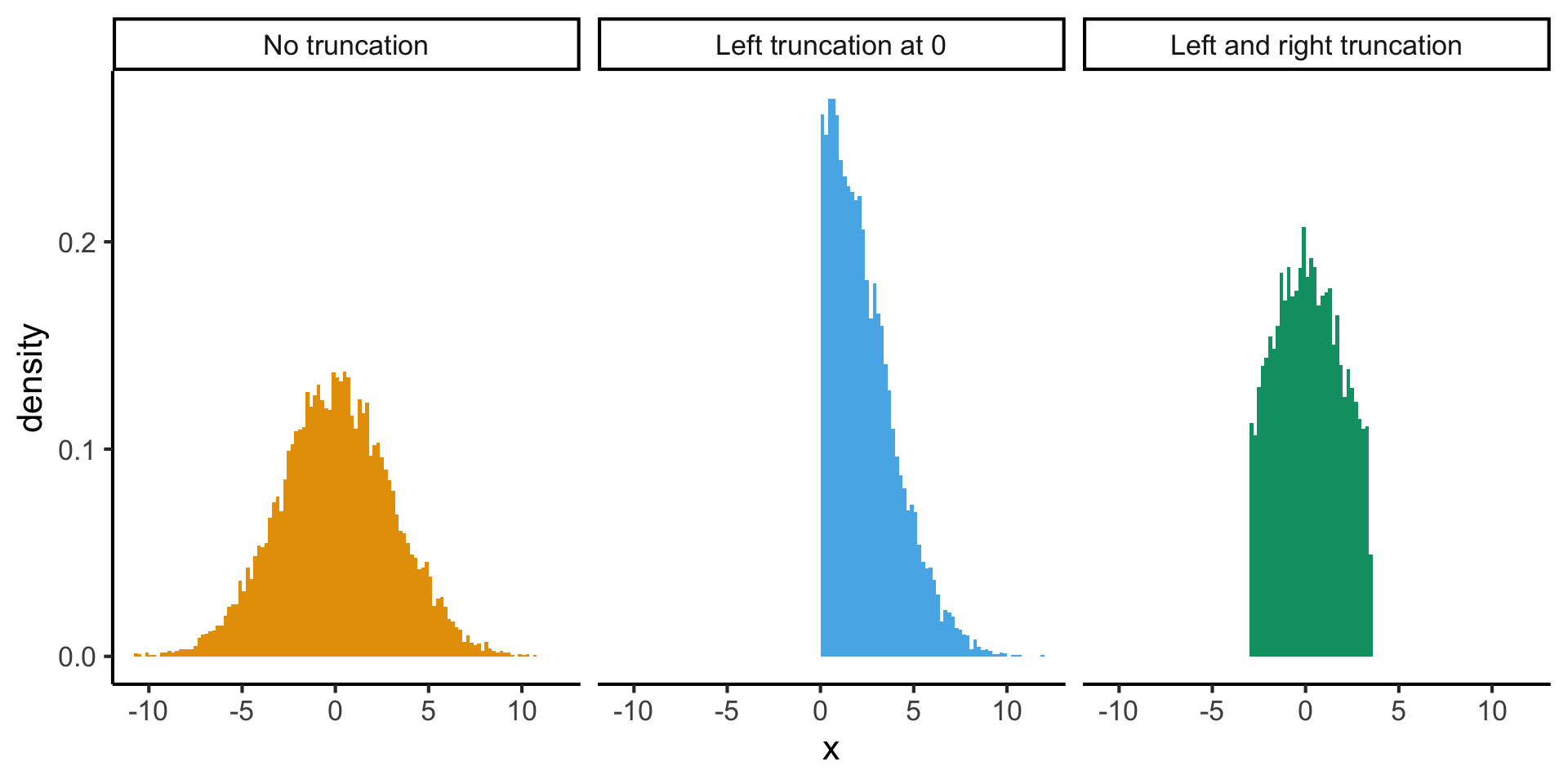
Adapted from simstudy package documentation

The Truncated Normal pdf

• Since we see a conditioning bar on the previous slide, we can infer what the pdf of this conditional distribution would look like. If \(X \sim \ddot{\mathcal{N}}(\mu, \sigma, a, b)\), then \(X\) has pdf

\[ f_X(x) = \frac{1}{\sigma}\cdot \frac{\varphi\left(\frac{x - \mu}{\sigma}\right)}{\Phi\left(\frac{b-\mu}{\sigma}\right) - \Phi\left(\frac{a - \mu}{\sigma}\right)} \approx \frac{\Pr(X \approx x, a < X < b)}{\Pr(a < X < b)} \]

• \(\varphi\) is the pdf of \(\mathcal{N}(0,1)\)
• \(\Phi\) is the CDF of \(\mathcal{N}(0,1)\)

(Note the lowercasing to describe pdfs and capitalizing to describe CDFs, even in Greek!)

Back to Working Backwards

• By definition of independence, we can obtain joint pdf \(f_{G,H}(g, h)\) by multiplying marginal pdf \(f_G(g)\) and marginal pdf \(f_H(h)\):

\[ \begin{align*} f_{G,H}(g, h) &= f_G(g) \cdot f_H(h) \\ &= \frac{1}{2} \cdot \left[ \frac{1}{0.1} \cdot \frac { \varphi\left(\frac{h - 0.5}{0.1}\right) } { \Phi\left(\frac{12-0.5}{0.1}\right) - \Phi\left(\frac{10 - 0.5}{0.1}\right) } \right] \end{align*} \]

Moving Forwards Again

• We’ve arrived at the case we had in discrete world, where we know the joint distribution!
• We can integrate wherever we took sums in the discrete case to obtain marginal pdfs:

\[ \begin{align*} f_G(g) &= \int_{0}^{1}f_{G,H}(g,h)\mathrm{d}h = \frac{1}{2}, \\ f_H(h) &= \int_{10}^{12}f_{G,H}(g, h)\mathrm{d}g = \frac{1}{0.1} \cdot \frac { \varphi\left(\frac{h - 0.5}{0.1}\right) } { \Phi\left(\frac{12 - 0.5}{0.1}\right) - \Phi\left(\frac{10 - 0.5}{0.1}\right) } \end{align*} \]

Conditional Distributions in Continuous World

• We can compute conditional pdfs by renormalizing
• Denominator is no longer integral of the distribution over all possible values (hence just the number \(1\)), but a ratio of joint distribution to marginal distribution values like:

\[ f_{H \mid G}(h | g) = \frac{f_{G,H}(g, h)}{f_G(g)}. \]

• At first this is magic… we can use the exact same equation from discrete world?!?
• But then you remember, continuous world was set up as a “hack”, using area under the curve between two points rather than height of the curve at a point to “port” discrete formulas into continuous world
• Think of how, when mathematicians hit the “wall” of solving \(x^2 + 1 = 0\)… They set up a new number \(i\) to work with these polynomials using “standard” algebra. Here we set up continuous pdf \(f_X(x)\) to work with continuous RVs using “standard” probability theory!

You Don’t Have To Stare Helplessly At Scary Math!

• Try to link the continuous equations back to their simpler discrete forms
• Work with the discrete forms to develop intuition, then
• Convert sums back into integrals once you’re ready

A Concrete Strategy

• Start by discretizing (“binning”) the possible values of a continuous RV to obtain a discrete RV:
  • Split \([10,12]\) into three equal-length bins, \([0,1]\) into two equal-length bins
  • Simulate \((G, H)\) pairs, sort into bins, plot joint / marginal / conditional distributions of binned data
• As you make bins thinner and thinner… 🤔

Thinking Through Specific Multivariate Distributions

• From \(2\) to \(N\) variables!

The Multinoulli Distribution

• May seem like a weird/contrived distribution, but is perfect for building intuition, as your first \(N\)-dimensional distribution (\(N > 2\))

• \(\mathbf{X}\) is a six-dimensional Vector-Valued RV, so that

  \[ \mathbf{X} = (X_1, X_2, X_3, X_4, X_5, X_6), \]

  where \(\mathcal{R}_{X_1} = \{0, 1\}, \mathcal{R}_{X_2} = \{0, 1\}, \ldots, \mathcal{R}_{X_6} = \{0, 1\}\)

• But, \(X_1, X_2, \ldots, X_6\) are not independent! In fact, they are so dependent that if one has value \(1\), the rest must have value \(0\) \(\leadsto\) we can infer the support of \(\mathbf{X}\):

  \[ \begin{align*} \mathcal{R}_{\mathbf{X}} = \{ &(1,0,0,0,0,0),(0,1,0,0,0,0),(0,0,1,0,0,0), \\ &(0,0,0,1,0,0),(0,0,0,0,1,0),(0,0,0,0,0,1)\} \end{align*} \]

• Lastly, need to define the probability that \(\mathbf{X}\) takes on any of these values. Let’s say \(\Pr(\mathbf{X} = \mathbf{v}) = \frac{1}{6}\) for all \(\mathbf{v} \in \mathcal{R}_{\mathbf{X}}\). Do we see the structure behind this contrived case?

• (For math major friends, there is an isomorphism afoot… For the rest, it’s an extremely inefficient way to model outcomes from rolling a fair die)

The Multivariate Normal Distribution

• We’ve already seen the matrix notation for writing the parameters of this distribution: \(\mathbf{X}_{[k \times 1]} \sim \mathcal{N}_k\left(\boldsymbol\mu_{[k \times 1]}, \Sigma_{[k \times k]}\right)\)
• Now we get to crack open the matrix notation for writing its pdf:

\[ f_\mathbf{X}(\mathbf{x}_{[k \times 1]}) = \underbrace{\left(\frac{1}{\sqrt{2\pi}}\right)^k \frac{1}{\sqrt{\det(\Sigma)}}}_{\text{Normalizing constants}} \exp\left(-\frac{1}{2}\underbrace{(\mathbf{x} - \boldsymbol\mu)^\top \Sigma^{-1} (\mathbf{x} - \boldsymbol\mu)}_{\text{Quadratic form}}\right) \]

• Try to squint your eyes while looking at the above and compare with…

pdf of \(\mathcal{N}(\mu,\sigma)\)

\[ f_X(v) = \frac{1}{\sigma\sqrt{2\pi}}\bigexp{-\frac{1}{2}\left(\frac{v - \mu}{\sigma}\right)^2} \]

Structure of \(\Sigma\)

\[ \begin{align*} \mathbf{\Sigma} &= \begin{bmatrix}\sigma_1^2 & \rho\sigma_1\sigma_2 \\ \rho\sigma_2\sigma_1 & \sigma_2^2\end{bmatrix} \\[0.1em] \implies \det(\Sigma) &= \sigma_1^2\sigma_2^2 - \rho^2\sigma_1^2\sigma_2^2 \\ &= \sigma_1^2\sigma_2^2(1-\rho^2) \end{align*} \]

Quadratic Forms

• Quadratic forms will seem scary until someone forces you to write out the matrix multiplication!
• Start with the 1D case: \(\mathbf{x} = [x_1]\), \(\boldsymbol\mu = [\mu_1]\), \(\Sigma = [\sigma^2]\). Then

\[ (\mathbf{x} - \boldsymbol\mu)^\top \Sigma^{-1} (\mathbf{x - \boldsymbol\mu}) = (x_1 - \mu_1)\frac{1}{\sigma^2}(x_1 - \mu_1) = \left(\frac{x_1 - \mu_1}{\sigma}\right)^2 ~ 🤯 \]

The 2D Case

• Let \(\mathbf{x} = \left[\begin{smallmatrix}x_1 \\ x_2\end{smallmatrix}\right]\), \(\boldsymbol\mu = \left[ \begin{smallmatrix}\mu_1 \\ \mu_2 \end{smallmatrix}\right]\), \(\Sigma\) as in previous slide. Then \(\mathbf{x} - \boldsymbol\mu = \left[ \begin{smallmatrix} x_1 - \mu_1 \\ x_2 - \mu_2 \end{smallmatrix} \right]\)
• Using what we know about \(2 \times 2\) matrix inversion,

\[ \Sigma^{-1} = \frac{1}{\det(\Sigma)}\left[ \begin{smallmatrix} \sigma_2^2 & -\rho \sigma_2\sigma_1 \\ -\rho \sigma_1\sigma_2 & \sigma_1^2\end{smallmatrix} \right] = \frac{1}{\sigma_1^2\sigma_2^2(1-\rho^2)}\left[ \begin{smallmatrix} \sigma_2^2 & -\rho \sigma_2\sigma_1 \\ -\rho \sigma_1\sigma_2 & \sigma_1^2\end{smallmatrix} \right] \]

• With \(\widetilde{\rho} \equiv 1 - \rho^2\), we can write everything as a bunch of matrix multiplications:

\[ \begin{align*} &(\mathbf{x} - \boldsymbol\mu)^\top \Sigma^{-1} (\mathbf{x} - \boldsymbol\mu) = \frac{1}{\sigma_1^2\sigma_2^2 \widetilde{\rho}} \begin{bmatrix}x_1 - \mu_1 & x_2 - \mu_2\end{bmatrix} \cdot \begin{bmatrix} \sigma_2^2 & -\rho \sigma_2\sigma_1 \\ -\rho \sigma_1\sigma_2 & \sigma_1^2\end{bmatrix} \cdot \begin{bmatrix}x_1 - \mu_1 \\ x_2 - \mu_2\end{bmatrix} \\ &= \frac{1}{\sigma_1^2\sigma_2^2 \widetilde{\rho}} \begin{bmatrix}(x_1-\mu_1)\sigma_2^2 - (x_2-\mu_2)\rho\sigma_1\sigma_2 & (x_2 - \mu_2)\sigma_1^2 - (x_1 - \mu_1)\rho\sigma_2\sigma_1 \end{bmatrix} \cdot \begin{bmatrix}x_1 - \mu_1 \\ x_2 - \mu_2\end{bmatrix} \\ &= \frac{1}{\sigma_1^2\sigma_2^2 \widetilde{\rho}} \left( (x_1-\mu_1)^2 \sigma_2^2 - (x_1 - \mu_1)(x_1 - \mu_2)\sigma_1\sigma_2 + (x_2 - \mu_2)^2 \sigma_1^2 - (x_1 - \mu_1)(x_2 - \mu_2)\sigma_2\sigma_1 \right) \\ &= \boxed{ \frac{1}{\widetilde{\rho}} \left( \left(\frac{x_1 - \mu_1}{\sigma_1}\right)^2 + \left(\frac{x_2 - \mu_2}{\sigma_2}\right)^2 - 2\rho\frac{(x_1 - \mu_1)(x_2 - \mu_2)}{\sigma_1\sigma_2} \right) } \end{align*} \]

The 2D Case In Its FINAL FORM

\[ f_{\mathbf{X}}(\mathbf{x}) = C \bigexp{ -\frac{1}{2(1-\rho^2)} \left( \left(\frac{x_1 - \mu_1}{\sigma_1}\right)^2 + \left(\frac{x_2 - \mu_2}{\sigma_2}\right)^2 - 2\rho\frac{(x_1 - \mu_1)(x_2 - \mu_2)}{\sigma_1\sigma_2} \right) } \]

where

\[ C = \frac{1}{2\pi\sigma_1\sigma_2\sqrt{1-\rho^2}}. \]

References

DeGroot, Morris H., and Mark J. Schervish. 2013. Probability and Statistics. Pearson Education.