Week 4: Continuous Distributions

DSAN 5100: Probabilistic Modeling and Statistical Computing
Section 01

Class Sessions

Author

Purna Gamage, Amineh Zadbood, and Jeff Jacobs

Published

Tuesday, September 16, 2025

Open slides in new window →

Probability Distributions in General

Discrete vs. Continuous

Discrete = “Easy mode”: Based (intuitively) on sets
\(\Pr(A)\): Four equally-likely marbles \(\{A, B, C, D\}\) in box, what is probability I pull out \(A\)?

library(tibble)
library(ggplot2)
disc_df <- tribble(
  ~x, ~y, ~label,
  0, 0, "A",
  0, 1, "B",
  1, 0, "C",
  1, 1, "D"
)
ggplot(disc_df, aes(x=x, y=y, label=label)) +
    geom_point(size=g_pointsize) +
    geom_text(
      size=g_textsize,
      hjust=1.5,
      vjust=-0.5
    ) +
    xlim(-0.5,1.5) + ylim(-0.5,1.5) +
    coord_fixed() +
    dsan_theme("quarter") +
    labs(
      title="Discrete Probability Space in N"
    )

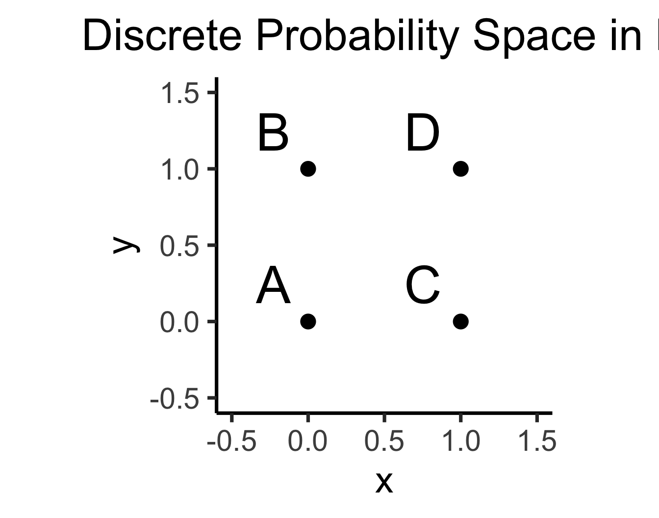
\[ \Pr(A) = \underset{\mathclap{\small \text{Probability }\textbf{mass}}}{\boxed{\frac{|\{A\}|}{|\Omega|}}} = \frac{1}{|\{A,B,C,D\}|} = \frac{1}{4} \]

Continuous = “Hard mode”: Based (intuitively) on areas
\(\Pr(A)\): Throw dart at random point in square, what is probability I hit \(\require{enclose}\enclose{circle}{\textsf{A}}\)?

library(ggforce)
ggplot(disc_df, aes(x=x, y=y, label=label)) +
    xlim(-0.5,1.5) + ylim(-0.5,1.5) +
    geom_rect(aes(xmin = -0.5, xmax = 1.5, ymin = -0.5, ymax = 1.5), fill=cbPalette[1], color="black", alpha=0.3) +
    geom_circle(aes(x0=x, y0=y, r=0.25), fill=cbPalette[2]) +
    coord_fixed() +
    dsan_theme("quarter") +
    geom_text(
      size=g_textsize,
      #hjust=1.75,
      #vjust=-0.75
    ) +
    geom_text(
      data=data.frame(label="Ω"),
      aes(x=-0.4,y=1.39),
      parse=TRUE,
      size=10
    ) +
    labs(
      title=expression("Continuous Probability Space in "*R^2)
    )

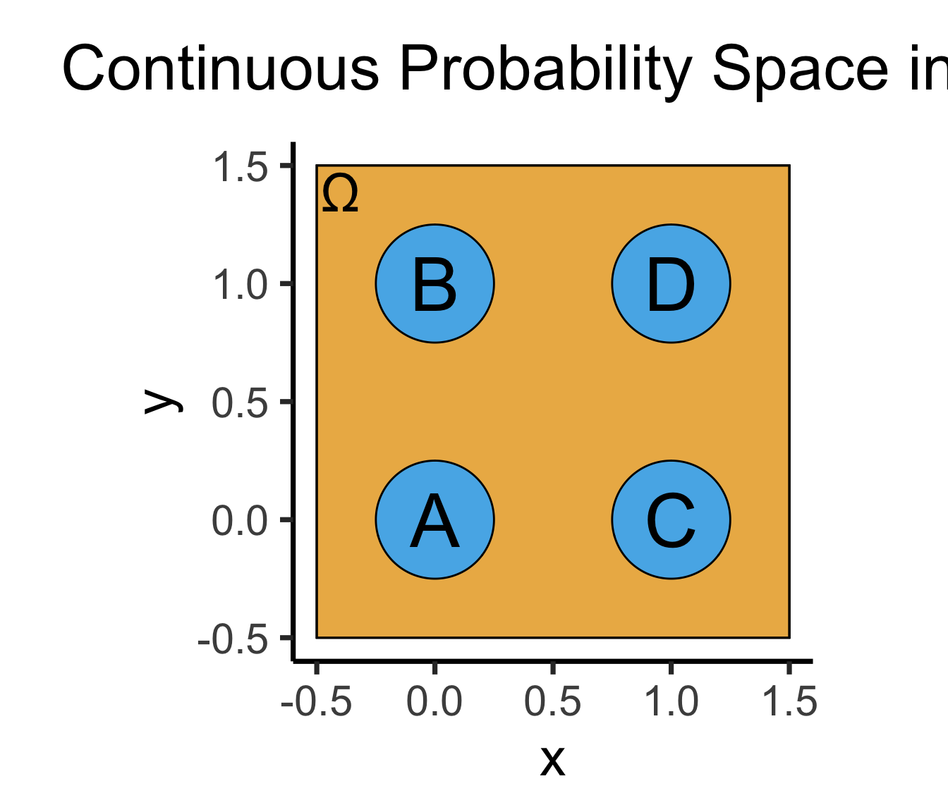
\[ \Pr(A) = \underset{\mathclap{\small \text{Probability }\textbf{density}}}{\boxed{\frac{\text{Area}(\{A\})}{\text{Area}(\Omega)}}} = \frac{\pi r^2}{s^2} = \frac{\pi \left(\frac{1}{4}\right)^2}{4} = \frac{\pi}{64} \]

The Technical Difference tl;dr

Countable Sets: Can be put into 1-to-1 correspondence with natural numbers \(\mathbb{N}\)
- What are you doing when you’re counting? Saying “first”, “second”, “third”, …
- You’re pairing each object with a natural number! \(\{(\texttt{a},1),(\texttt{b},2),\ldots,(\texttt{z},26)\}\)
Uncountable Sets: Can’t be put into 1-to-1 correspondence with natural numbers.
\(\mathbb{R}\) is uncountable. Intuition: Try counting the real numbers. Proof \[ \text{Assume }\exists \, (f: \mathbb{R} \leftrightarrow \mathbb{N}): \begin{array}{|c|c|c|c|c|c|c|}\hline \mathbb{R} & & & & & & \Leftrightarrow \mathbb{N} \\ \hline \color{orange}{3} & . & 1 & 4 & 1 & \cdots & \Leftrightarrow 1 \\\hline 4 & . & \color{orange}{9} & 9 & 9 & \cdots & \Leftrightarrow 2 \\\hline 0 & . & 1 & \color{orange}{2} & 3 & \cdots &\Leftrightarrow 3 \\\hline 1 & . & 2 & 3 & \color{orange}{4} & \cdots & \Leftrightarrow 4 \\\hline \vdots & \vdots & \vdots & \vdots & \vdots & \ddots & \vdots \\\hline \end{array} \overset{\color{blue}{y_{[i]}} = \color{orange}{x_{[i]}} \overset{\mathbb{Z}_{10}}{+} 1}{\underset{😈}{\longrightarrow}} \color{blue}{y = 4.035 \ldots} \Leftrightarrow \; ? \]

Fun math challenge: Is \(\mathbb{Q}\) countable? See this appendix slide for why the answer is yes, despite the fact that \(\forall x, y \in \mathbb{Q} \left[ \frac{x+y}{2} \in \mathbb{Q} \right]\)❗️ The method used in the above proof is called Cantor diagonalization

The Practical Difference

This part of the course (discrete probability): \(\Pr(X = v), v \in \mathcal{R}_X \subseteq \mathbb{N}\)
- Example: \(\Pr(\)\() = \Pr(X = 3), 3 \in \{1,2,3,4,5,6\} \subseteq \mathbb{N}\)
Next part of the course (continuous probability): \(\Pr(X \in V), V \subseteq \mathbb{R}\)
- Example: \(\Pr(X \geq 2\pi) = \Pr(X \in [\pi,\infty)), [\pi,\infty) \subseteq \mathbb{R}\)
Why do they have to be in separate parts?

\[ \Pr(X \underset{\substack{\uparrow \\ 🚩}}{=} 2\pi) = \frac{\text{Area}(\overbrace{2\pi}^{\mathclap{\small \text{Single point}}})}{\text{Area}(\underbrace{\mathbb{R}}_{\mathclap{\small \text{(Uncountably) Infinite set of points}}})} = 0 \]

The CDF Unifies the Two Worlds!

Cumulative Distribution Function (CDF): \(F_X(v) = \Pr(X \leq v)\)¹
For discrete RV \(X\) (\(\mathcal{R}_X \cong \mathbb{N}\)), Probability Mass Function (pmf) \(p_X(v)\): \[ \begin{align*} p_X(v) &\definedas \Delta F_X(v) \definedas F_X(v) - F_X(v - 1) = \underset{\text{Meaningful}}{\boxed{\Pr(X = v)}} \\ \implies F_X(v) &= \sum_{\{w \in \mathcal{R}_X: \; w \leq v\}}p_X(w) = \underset{\text{Meaningful}}{\boxed{\Pr(X \leq v)}} \end{align*} \]
For continuous RV \(X\) (\(\mathcal{R}_X \subseteq \mathbb{R}\)), Probability Density Function (pdf) \(f_X(v)\): \[ \begin{align*} f_X(v) &\definedas \frac{d}{dx}F_X(v) \definedas \lim_{h \rightarrow 0}\frac{F(x + h) - F(x)}{h} = \underset{\text{Not Meaningful}}{\boxed{\; ? \;}} \\ \implies F_X(v) &= \int_{-\infty}^v f_X(w)dw = \underset{\text{Meaningful}}{\boxed{\Pr(X \leq v)}} \end{align*} \]

Probability Density \(\neq\) Probability

☠️BEWARE☠️: \(f_X(v) \neq \Pr(X = v)\)!
Long story short, for continuous variables, \(\Pr(X = v)\) is just always \(0\)[^measurezero]
Hence, we instead construct a pdf \(f_X(v)\) whose sole purpose is to allow us to calculate \(\Pr(X \in [a,b])\) by integrating!
- \(f_X(v)\) is whatever satisfies \(\Pr(X \in [a,b]) = \int_{a}^bf_X(v)dv\), and nothing more
i.e., instead of \(p_X(v) = \Pr(X = v)\) from discrete world, the relevant function here is \(f_X(v)\), the probability density of \(X\) at \(v\).

Scary math zone

For intuition: think of \(X \sim \mathcal{U}(0,10) \implies \Pr(X = \pi) = \frac{|\{v \in \mathbb{R}:\; v = \pi\}|}{|\mathbb{R}|} = \frac{1}{2^{\aleph_0}} \approx 0\). That is, finding the \(\pi\) needle in the \(\mathbb{R}\) haystack is a one-in-\(\left(\infty^\infty\right)\) event.
Issue even if \(\mathcal{R}_X\) countably infinite, like \(\mathcal{R}_X = \mathbb{N}\): \(\Pr(X = 3) = \frac{|\{x \in \mathbb{N} : \; x = 3\}|}{|\mathbb{N}|} = \frac{1}{\aleph_0}\). Finding the \(3\) needle in the \(\mathbb{N}\) haystack is a one-in-\(\infty\) event

Common Discrete Distributions

Bernoulli
Binomial
Geometric

Bernoulli Distribution

Single trial with two outcomes, “success” (1) or “failure” (0): basic model of a coin flip (heads = 1, tails = 0)
\(X \sim \text{Bern}({\color{purple} p}) \implies \mathcal{R}_X = \{0,1\}, \; \Pr(X = 1) = {\color{purple}p}\).

library(ggplot2)
library(tibble)
bern_tibble <- tribble(
  ~Outcome, ~Probability, ~Color,
  "Failure", 0.2, cbPalette[1],
  "Success", 0.8, cbPalette[2]
)
ggplot(data = bern_tibble, aes(x=Outcome, y=Probability)) +
  geom_bar(aes(fill=Outcome), stat = "identity") +
  dsan_theme("half") +
  labs(
    y = "Probability Mass"
  ) +
  scale_fill_manual(values=c(cbPalette[1], cbPalette[2])) +
  remove_legend()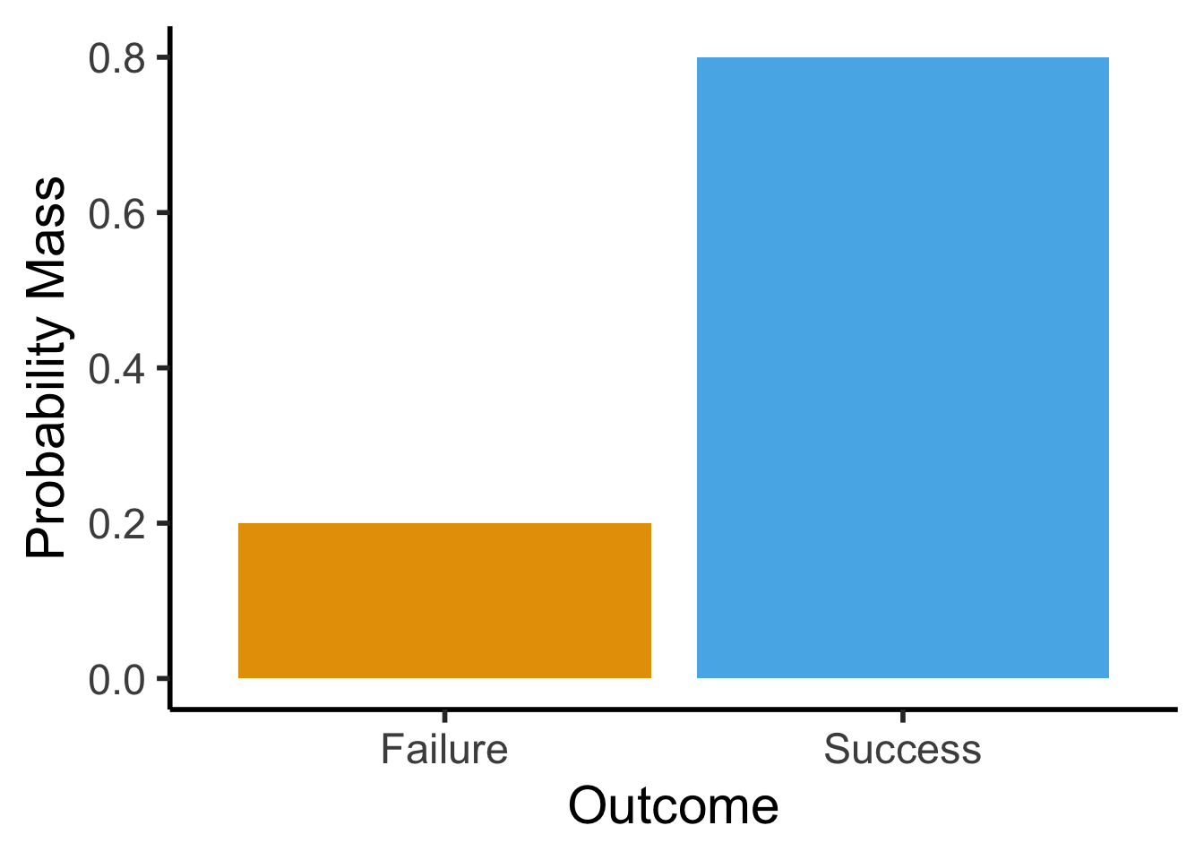

Binomial Distribution

Number of successes in \({\color{purple}N}\) Bernoulli trials. \(X \sim \text{Binom}({\color{purple}N},{\color{purple}k},{\color{purple}p}) \implies \mathcal{R}_X = \{0, 1, \ldots, N\}\)
- \(\Pr(X = k) = \binom{N}{k}p^k(1-p)^{N-k}\): probability of \(k\) successes out of \(N\) trials.
- \(\binom{N}{k} = \frac{N!}{k!(N-k)!}\): “Binomial coefficient”. How many groups of size \(k\) can be formed?²

Visualizing the Binomial

Code

k <- seq(0, 10)
prob <- dbinom(k, 10, 0.5)
bar_data <- tibble(k, prob)
ggplot(bar_data, aes(x=k, y=prob)) +
  geom_bar(stat="identity", fill=cbPalette[1]) +
  labs(
    title="Binomial Distribution, N = 10, p = 0.5",
    y="Probability Mass"
  ) +
  scale_x_continuous(breaks=seq(0,10)) +
  dsan_theme("half")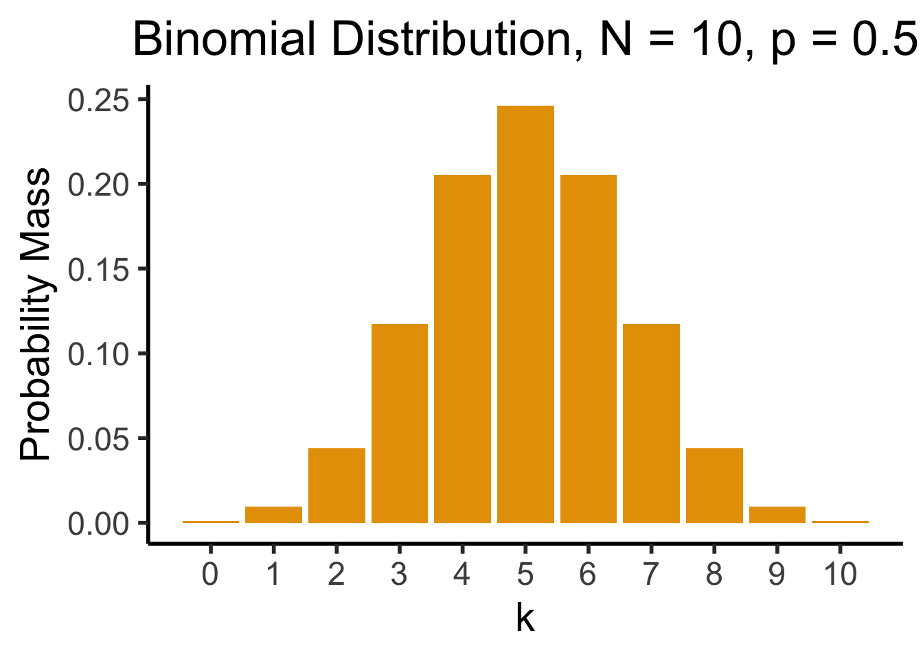

So who can tell me, from this plot, the approximate probability of getting 4 heads when flipping a coin 10 times?

Multiple Classes: Multinomial Distribution

Bernoulli only allows two outcomes: success or failure.
What if we’re predicting soccer match outcomes?
- \(X_i \in \{\text{Win}, \text{Loss}, \text{Draw}\}\)
Categorical Distribution: Generalizes Bernoulli to \(k\) possible outcomes. \(X \sim \text{Categorical}(\mathbf{p} = \{p_1, p_2, \ldots, p_k\}), \sum_{i=1}^kp_i = 1\).
- \(\Pr(X = k) = p_k\)
Multinomial Distribution: Generalizes Binomial to \(k\) possible outcomes.
\(\mathbf{X} \sim \text{Multinom}(N,k,\mathbf{p}=\{p_1,p_2,\ldots,p_k\}), \sum_{i=1}^kp_i=1\)
- \(\Pr(\mathbf{X} = \{x_1,x_2\ldots,x_k\}) = \frac{N!}{x_1!x_2!\cdots x_k!}p_1^{x_1}p_2^{x_2}\cdots p_k^{x_k}\)
- \(\Pr(\text{30 wins}, \text{4 losses}, \text{4 draws}) = \frac{38!}{30!4!4!}p_{\text{win}}^{30}p_{\text{lose}}^4p_{\text{draw}}^4\).
- \(\leadsto\) “Multinomial Coefficient”: \(\binom{38}{30,4,4} = \frac{38!}{30!4!4!}\)

Geometric Distribution

Likelihood that we need \({\color{purple}k}\) trials to get our first success. \(X \sim \text{Geom}({\color{purple}k},{\color{purple}p}) \implies \mathcal{R}_X = \{1, 2, \ldots\}\)
- \(\Pr(X = k) = \underbrace{(1-p)^{k-1}}_{\small k - 1\text{ failures}}\cdot \underbrace{p}_{\mathclap{\small \text{success}}}\)
- Probability of \(k\) trials before first success

library(ggplot2)
k <- seq(0, 8)
prob <- dgeom(k, 0.5)
bar_data <- tibble(k, prob)
ggplot(bar_data, aes(x = k, y = prob)) +
    geom_bar(stat = "identity", fill = cbPalette[1]) +
    labs(
        title = "Geometric Distribution, p = 0.5",
        y = "Probability Mass"
    ) +
    scale_x_continuous(breaks = seq(0, 8)) +
    dsan_theme("half")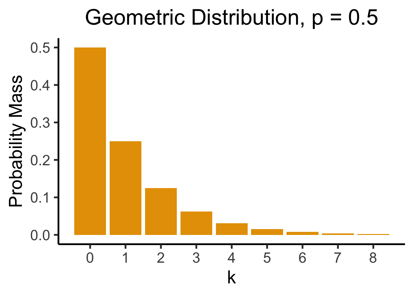

Less Common (But Important) Distributions

Discrete Uniform: \(N\) equally-likely outcomes
- \(X \sim U\{{\color{purple}a},{\color{purple}b}\} \implies \mathcal{R}_X = \{a, a+1, \ldots, b\}, \Pr(X = k) = \frac{1}{{\color{purple}b} - {\color{purple}a} + 1}\)
Beta: \(X \sim \text{Beta}({\color{purple}\alpha}, {\color{purple}\beta})\): conjugate prior for Bernoulli, Binomial, and Geometric dists.
- Intuition: If we use Beta to encode our prior hypothesis, then observe data drawn from Binomial, distribution of our updated hypothesis is still Beta.
- \(\underbrace{\Pr(\text{biased}) = \Pr(\text{unbiased})}_{\text{Prior: }\text{Beta}({\color{purple}\alpha}, {\color{purple}\beta})} \rightarrow\) Observe \(\underbrace{\frac{8}{10}\text{ heads}}_{\text{Data}} \rightarrow \underbrace{\Pr(\text{biased}) = 0.65}_{\text{Posterior: }\text{Beta}({\color{purple}\alpha + 8}, {\color{purple}\beta + 2})}\)
Dirichlet: \(\mathbf{X} = (X_1, X_2, \ldots, X_K) \sim \text{Dir}({\color{purple} \boldsymbol\alpha})\)
- \(K\)-dimensional extension of Beta (thus, conjugate prior for Multinomial)

We can now use \(\text{Beta}(\alpha + 8, \beta + 2)\) as a prior for our next set of trials (encoding our knowledge up to that point), and update further once we know the results (to yet another Beta distribution).

Interactive Visualizations!

Seeing Theory, Brown University

Continuous Probability

(With some final reminders first!)

What Things Have Distributions?

Answer: Random Variables
Meaning: \(\mathcal{N}(0, 1)\) on its own is a “template”, an exhibit at a museum within a glass case
To start using it, e.g., to generate random values, we need to consider a particular RV \(X \sim \mathcal{N}(0,1)\), then generate values on basis of this template:
- \(X = 0\) more likely than \(X = 1\) or \(X = -1\),
- \(X = 1\) more likely than \(X = 2\) or \(X = -2\),
- and so on

CDFs/pdfs/pmfs: What Are They?

Functions which answer questions about a Random Variable (\(X\) in this case) with respect to a non-random value (\(v\) in this case, for “value”)
CDF: What is probability that \(X\) takes on a value less than or equal to \(v\)?

\[ F_X(v) \definedas \Pr(X \leq v) \]

pmf: What is the probability of this exact value? (Discrete only)

\[ p_X(v) \definedas \Pr(X = v) \]

pdf: 🙈 …It’s the thing you integrate to get the CDF

\[ f_X(v) \definedas \frac{d}{dv}F_X(v) \iff \int_{-\infty}^{v} f_X(v)dv = F_X(v) \]

CDFs/pdfs/pmfs: Why Do We Use Them?

CDF is like the “API” that allows you to access all of the information about the distribution (pdf/pmf is derived from the CDF)
Example: we know there’s some “thing” called the Exponential Distribution…
How do we use this distribution to understand a random variable \(X \sim \text{Exp}(\lambda)\)?
- Answer: the CDF of \(X\)!
- Since all exponentially-distributed RVs have the same pdf (with different \(\lambda\) values plugged in), we can call this pdf “the” exponential distribution
Say we want to find the median of \(X\): The median is the number(s) \(m\) satisfying

\[ \Pr(X \leq m) = \frac{1}{2} \]

How can we find this? What “tool” do we use to figure this out about \(X\)?

Finding a Median via the CDF

Median of a Random Variable \(X\)

The median of a random variable \(X\) with some CDF \(F_X(v_X)\) is the [set of] numbers \(m\) for which the probability that \(X\) is lower than \(m\) is \(\frac{1}{2}\):

\[ \begin{align*} \text{Median}(X) &= \left\{m \left| F_X(m) = \frac{1}{2} \right. \right\} \\ &= \left\{m \left| \int_{-\infty}^{m}f_X(v_X)dv_X = \frac{1}{2} \right. \right\} \end{align*} \]

(If you’re wondering why we start with the median rather than the more commonly-used mean: it’s specifically because I want you to get used to calculating general functions \(f(X)\) of a random variable \(X\). It’s easy to just e.g. learn how to compute the mean \(\expect{X}\) and forget that this is only one of many possible choices for \(f(X)\).)

Median via CDF Example

Example: If \(X \sim \text{Exp}(\param{\lambda})\),

\[ F_X(v) = 1 - e^{-\lambda v} \]

So we want to solve for \(m\) in

\[ F_X(m) = \frac{1}{2} \iff 1 - e^{-\lambda m} = \frac{1}{2} \]

Step-by-Step

\[ \begin{align*} 1 - e^{-\lambda m} &= \frac{1}{2} \\ \iff e^{-\lambda m} &= \frac{1}{2} \\ \iff \ln\left[e^{-\lambda m}\right] &= \ln\left[\frac{1}{2}\right] \\ \iff -\lambda m &= -\ln(2) \\ \iff m &= \frac{\ln(2)}{\lambda} %3x = 19-2y \; \llap{\mathrel{\boxed{\phantom{m = \frac{\ln(2)}{\lambda}}}}}. \end{align*} \]

Top Secret Fun Fact

Every Discrete Distribution is [technically, in a weird way] a Continuous Distribution!

Same intuition as: every natural number is a real number, but converse not true
Marbles: Let \(X\) be a RV defined s.t. \(X(A) = 1\), \(X(B) = 2\), \(X(C) = 3\), \(X(D) = 4\). Then pmf for \(X\) is \(p_X(i) = \frac{1}{4}\) for \(i \in \{1, 2, 3, 4\}\).
We can then use the Dirac delta function \(\delta(v)\) to define a continuous pdf

\[ f_X(v) = \sum_{i \in \mathcal{R}_X}p_X(i)\delta(v - i) = \sum_{i=1}^4p_X(i)\delta(v-i) = \frac{1}{4}\sum_{i=1}^4 \delta(v - i) \]

and use either the (discrete) pmf \(p_X(v)\) or (continuous) pdf \(f_X(v)\) to describe \(X\):

\[ \begin{align*} \overbrace{\Pr(X \leq 3)}^{\text{CDF}} &= \sum_{i=1}^3\overbrace{p_X(i)}^{\text{pmf}} = \frac{1}{4} + \frac{1}{4} + \frac{1}{4} = \frac{3}{4} \\ \underbrace{\Pr(X \leq 3)}_{\text{CDF}} &= \int_{-\infty}^{3} \underbrace{f_X(v)}_{\text{pdf}} = \frac{1}{4}\int_{-\infty}^{3} \sum_{i = 1}^{4}\overbrace{\delta(v-i)}^{\small 0\text{ unless }v = i}dv = \frac{3}{4} \end{align*} \]

Common Continuous Distributions

Normal: The friend who shows up everywhere
Uniform: The stable, reliable friend
Exponential: Good days and bad days
Cauchy: Toxic af, stay away ☠️

[Recall] Binomial Distribution

Code

k <- seq(0, 10)
prob <- dbinom(k, 10, 0.5)
bar_data <- tibble(k, prob)
ggplot(bar_data, aes(x=k, y=prob)) +
  geom_bar(stat="identity", fill=cbPalette[1]) +
  labs(
    title="Binomial Distribution, N = 10, p = 0.5",
    y="Probability Mass"
  ) +
  scale_x_continuous(breaks=seq(0,10)) +
  dsan_theme("half")

The Emergence of Order

Who can guess the state of this process after 10 steps, with 1 person?
10 people? 50? 100? (If they find themselves on the same spot, they stand on each other’s heads)
100 steps? 1000?

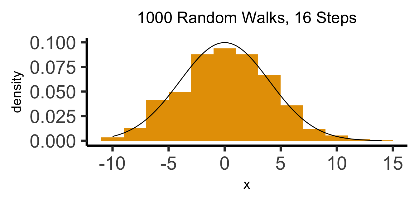
The Result: 16 Steps

Code

library(tibble)
library(ggplot2)
library(ggExtra)
library(dplyr)
library(tidyr)
# From McElreath!
gen_histo <- function(reps, num_steps) {
  support <- c(-1,1)
  pos <-replicate(reps, sum(sample(support,num_steps,replace=TRUE,prob=c(0.5,0.5))))
  #print(mean(pos))
  #print(var(pos))
  pos_df <- tibble(x=pos)
  clt_distr <- function(x) dnorm(x, 0, sqrt(num_steps))
  plot <- ggplot(pos_df, aes(x=x)) +
    geom_histogram(aes(y = after_stat(density)), fill=cbPalette[1], binwidth = 2) +
    stat_function(fun = clt_distr) +
    dsan_theme("quarter") +
    theme(title=element_text(size=16)) +
    labs(
      title=paste0(reps," Random Walks, ",num_steps," Steps")
    )
  return(plot)
}
gen_walkplot <- function(num_people, num_steps, opacity=0.15) {
  support <- c(-1, 1)
  # Unique id for each person
  pid <- seq(1, num_people)
  pid_tib <- tibble(pid)
  pos_df <- tibble()
  end_df <- tibble()
  all_steps <- t(replicate(num_people, sample(support, num_steps, replace = TRUE, prob = c(0.5, 0.5))))
  csums <- t(apply(all_steps, 1, cumsum))
  csums <- cbind(0, csums)
  # Last col is the ending positions
  ending_pos <- csums[, dim(csums)[2]]
  end_tib <- tibble(pid = seq(1, num_people), endpos = ending_pos, x = num_steps)
  # Now convert to tibble
  ctib <- as_tibble(csums, name_repair = "none")
  merged_tib <- bind_cols(pid_tib, ctib)
  long_tib <- merged_tib %>% pivot_longer(!pid)
  # Convert name -> step_num
  long_tib <- long_tib %>% mutate(step_num = strtoi(gsub("V", "", name)) - 1)
  # print(end_df)
  grid_color <- rgb(0, 0, 0, 0.1)

  # And plot!
  walkplot <- ggplot(
      long_tib,
      aes(
          x = step_num,
          y = value,
          group = pid,
          # color=factor(label)
      )
  ) +
      geom_line(linewidth = g_linesize, alpha = opacity, color = cbPalette[1]) +
      geom_point(data = end_tib, aes(x = x, y = endpos), alpha = 0) +
      scale_x_continuous(breaks = seq(0, num_steps, num_steps / 4)) +
      scale_y_continuous(breaks = seq(-20, 20, 10)) +
      dsan_theme("quarter") +
      theme(
          legend.position = "none",
          title = element_text(size = 16)
      ) +
      theme(
          panel.grid.major.y = element_line(color = grid_color, linewidth = 1, linetype = 1)
      ) +
      labs(
          title = paste0(num_people, " Random Walks, ", num_steps, " Steps"),
          x = "Number of Steps",
          y = "Position"
      )
}
wp1 <- gen_walkplot(500, 16, 0.05)
ggMarginal(wp1, margins = "y", type = "histogram", yparams = list(binwidth = 1))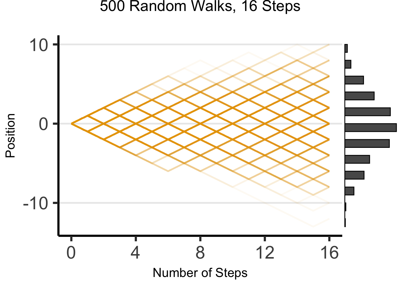

The Result: 64 Steps

Code

library(ggExtra)
wp2 <- gen_walkplot(5000,64,0.008) +
  ylim(-30,30)
ggMarginal(wp2, margins = "y", type = "histogram", yparams = list(binwidth = 1))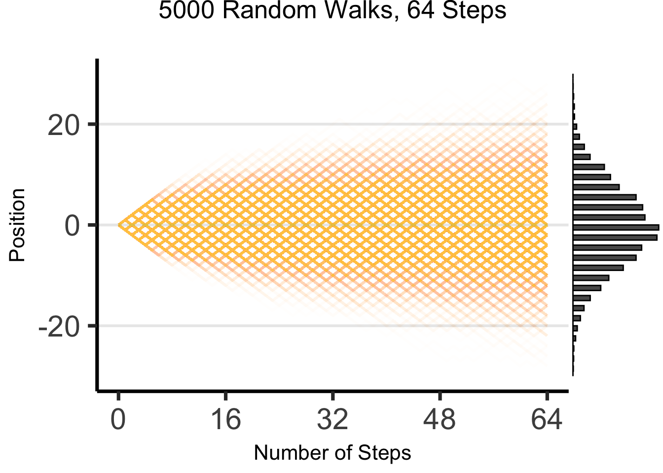

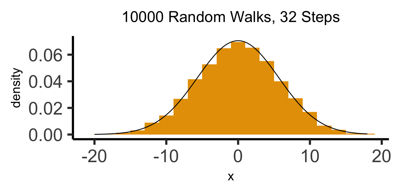
What’s Going On Here?

(Stay tuned for Markov processes \(\overset{t \rightarrow \infty}{\leadsto}\) Stationary distributions!)

Properties of the Normal Distribution

If \(X \sim \mathcal{N}(\param{\mu}, \param{\theta})\), then \(X\) has pdf \(f_X(v)\) defined by

\[ f_X(v) = \frac{1}{\sigma\sqrt{2\pi}}\bigexp{-\frac{1}{2}\left(\frac{v - \mu}{\sigma}\right)^2} \]

I hate memorizing as much as you do, I promise 🥴
The important part (imo): this is the most conservative out of all possible (symmetric) prior distributions defined on \(\mathbb{R}\) (defined from \(-\infty\) to \(\infty\))

“Most Conservative” How?

Of all possible distributions with mean \(\mu\), variance \(\sigma^2\), \(\mathcal{N}(\mu, \sigma^2)\) is the entropy-maximizing distribution
Roughly: using any other distribution (implicitly/secretly) imports additional information beyond the fact that mean is \(\mu\) and variance is \(\sigma^2\)
Example: let \(X\) be an RV. If we know mean is \(\mu\), variance is \(\sigma^2\), but then we learn that \(X \neq 3\), or \(X\) is even, or the 15th digit of \(X\) is 7, can update \(\mathcal{N}(\mu,\sigma^2)\) to derive a “better” distribution (incorporating this additional info)

The Takeaway

Given info we know, we can find a distribution that “encodes” only this info
More straightforward example: if we only know that the value is something in the range \([a,b]\), entropy-maximizing distribution is the Uniform Distribution

If We Know	And We Know	(Max-Entropy) Distribution Is…
\(\text{Mean}[X] = \mu\)	\(\text{Var}[X] = \sigma^2\)	\(X \sim \mathcal{N}(\mu, \sigma^2)\)
\(\text{Mean}[X] = \lambda\)	\(X \geq 0\)	\(X \sim \text{Exp}\left(\frac{1}{\lambda}\right)\)
\(X \geq a\)	\(X \leq b\)	\(X \sim \mathcal{U}[a,b]\)

[Recall] Discrete Uniform Distribution

Code

library(tibble)
bar_data <- tribble(
  ~x, ~prob,
  1, 1/6,
  2, 1/6,
  3, 1/6,
  4, 1/6,
  5, 1/6,
  6, 1/6
)
ggplot(bar_data, aes(x=x, y=prob)) +
  geom_bar(stat="identity", fill=cbPalette[1]) +
  labs(
    title="Discrete Uniform pmf: a = 1, b = 6",
    y="Probability Mass",
    x="Value"
  ) +
  scale_x_continuous(breaks=seq(1,6)) +
  dsan_theme("half")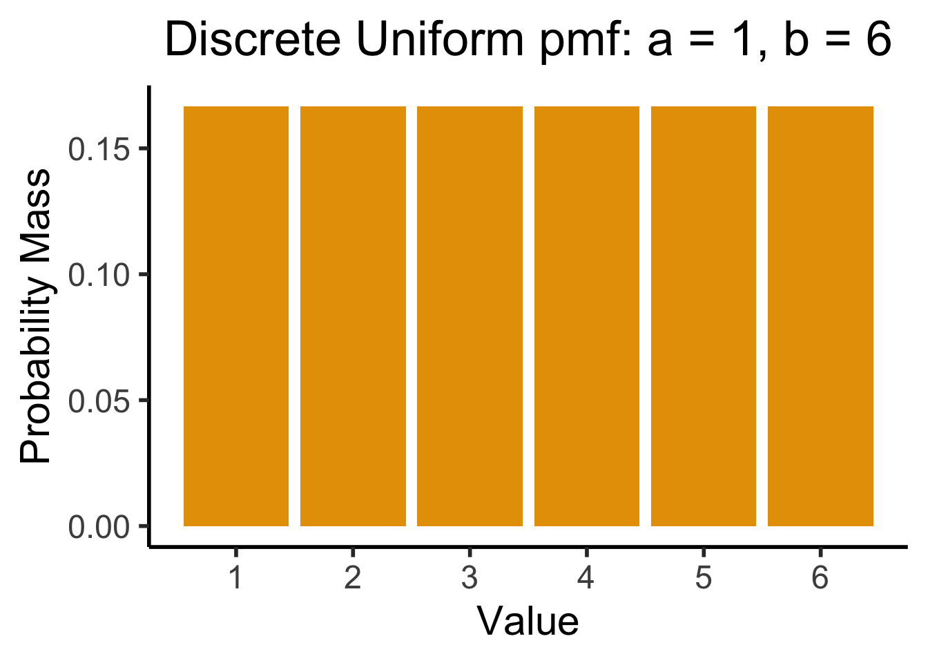

Continuous Uniform Distribution

If \(X \sim \mathcal{U}[a,b]\), then intuitively \(X\) is a value randomly selected from within \([a,b]\), with all values equally likely.
Discrete case: what we’ve been using all along (e.g., dice): if \(X \sim \mathcal{U}\{1,6\}\), then

\[ \Pr(X = 1) = \Pr(X = 2) = \cdots = \Pr(X = 6) = \frac{1}{6} \]

For continuous case… what do we put in the denominator? \(X \sim \mathcal{U}[1,6] \implies \Pr(X = \pi) = \frac{1}{?}\)…
- Answer: \(\Pr(X = \pi) = \frac{1}{|[1,6]|} = \frac{1}{\aleph_0} = 0\)

Constructing the Uniform CDF

We were ready for this! We already knew \(\Pr(X = v) = 0\) for continuous \(X\)
So, we forget about \(\Pr(X = v)\), and focus on \(\Pr(X \in [v_0, v_1])\).
In 2D (dartboard) we had \(\Pr(X \in \circ) = \frac{\text{Area}(\circ)}{\text{Area}(\Omega)}\), so here we should have

\[ P(X \in [v_0,v_1]) = \frac{\text{Length}([v_0,v_1])}{\text{Length}([1,6])} \]

And indeed, the CDF of \(X\) is \(\boxed{F_X(v) = \Pr(X \leq v) = \frac{v-a}{b-a}}\), so that

\[ \Pr(X \in [v_0,v_1]) = F_X(v_1) - F_X(v_0) = \frac{v_1-a}{b-a} - \frac{v_0-a}{b-a} = \frac{v_1 - v_0}{b-a} \]

Since \(a = 1\), \(b = 6\) in our example, \(\Pr(X \in [v_0,v_1]) = \frac{v_1-v_0}{6-1} = \frac{\text{Length}([v_0,v_1])}{\text{Length}([1,6])} \; ✅\)

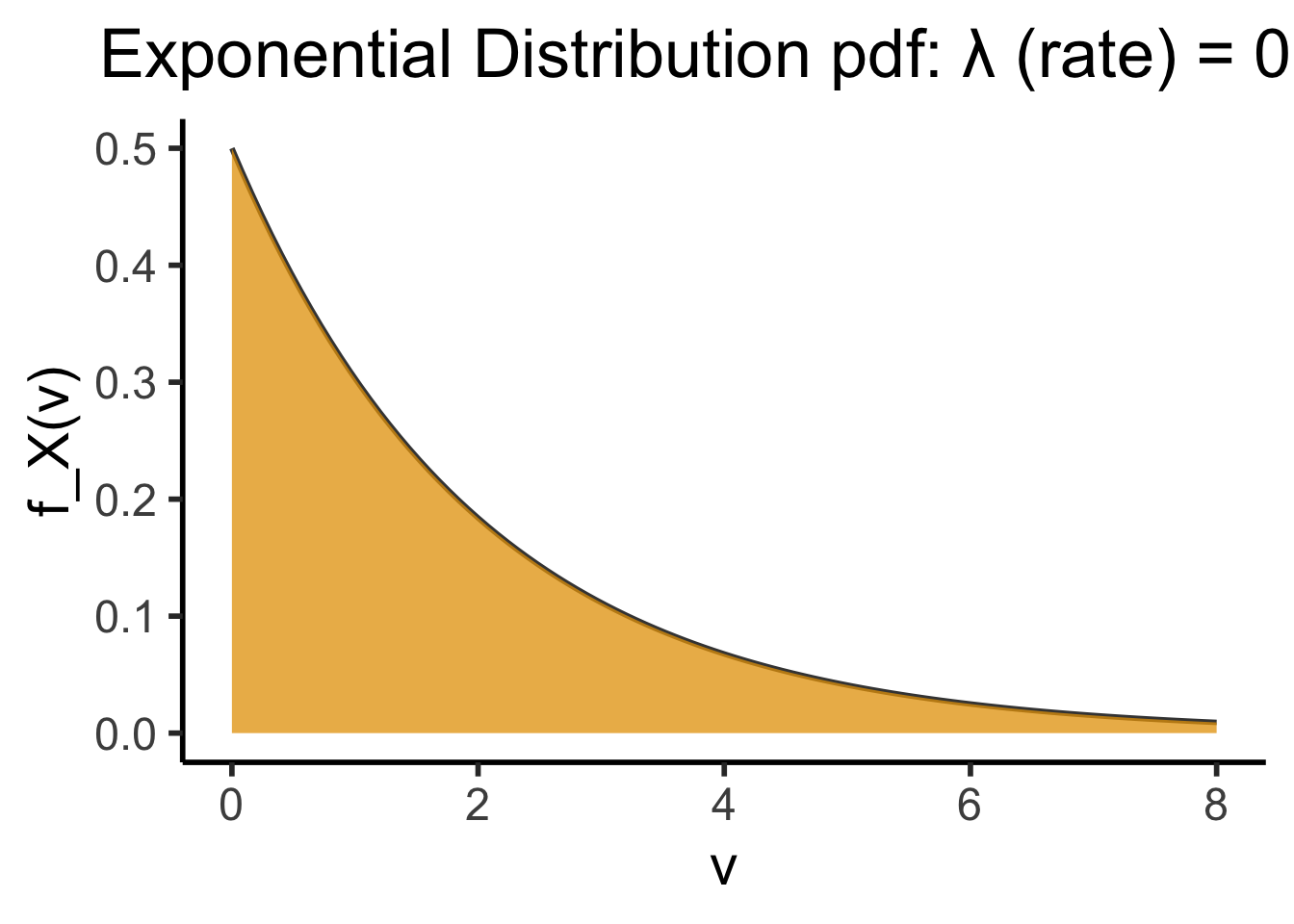
Exponential Distribution

Recall the (discrete) Geometric Distribution:

Code

library(ggplot2)
k <- seq(0, 8)
prob <- dgeom(k, 0.5)
bar_data <- tibble(k, prob)
ggplot(bar_data, aes(x = k, y = prob)) +
    geom_bar(stat = "identity", fill = cbPalette[1]) +
    labs(
        title = "Geometric Distribution pmf: p = 0.5",
        y = "Probability Mass"
    ) +
    scale_x_continuous(breaks = seq(0, 8)) +
    dsan_theme("half")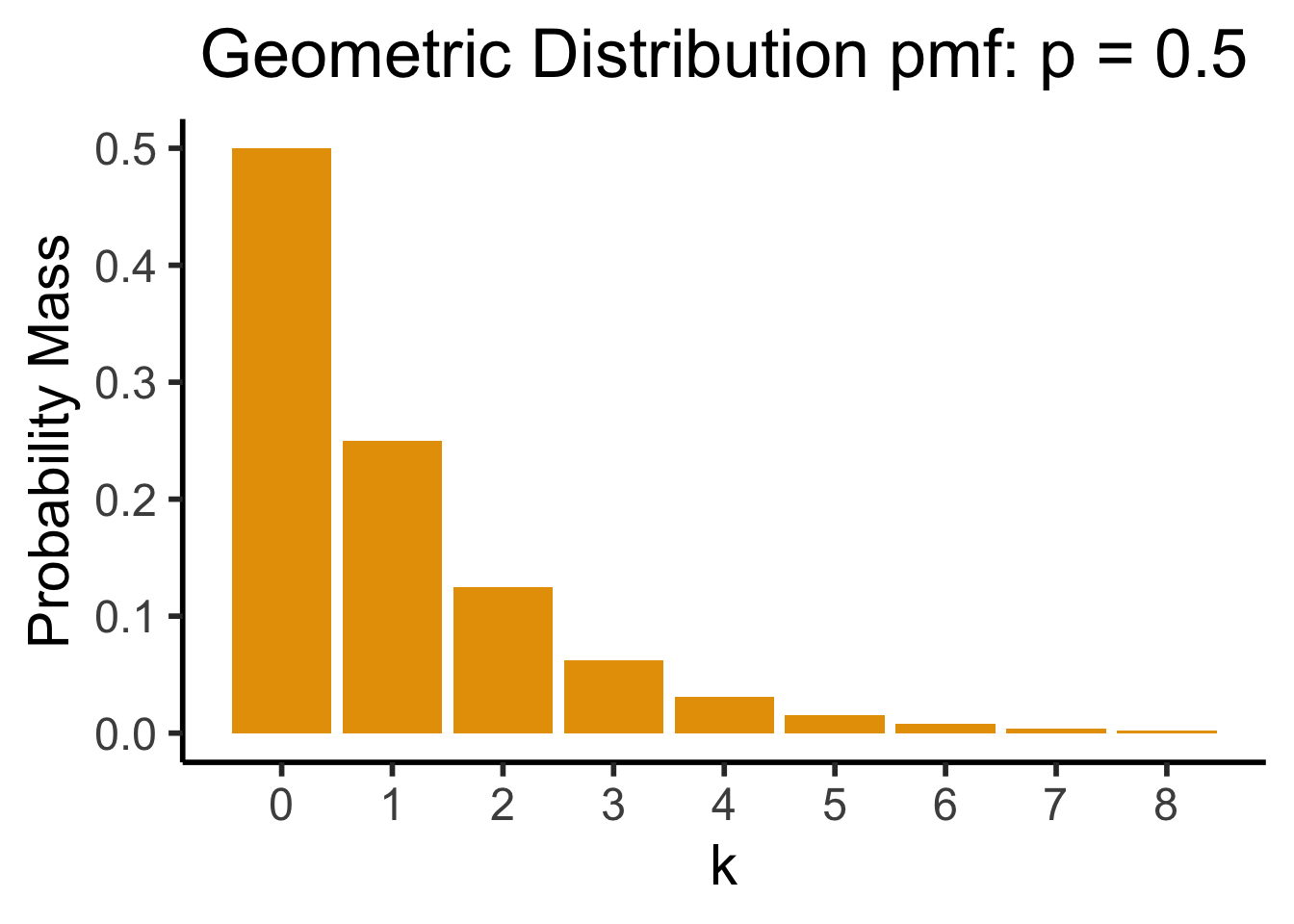

Now In Continuous Form!

Code

my_dexp <- function(x) dexp(x, rate = 1/2)
ggplot(data.frame(x=c(0,8)), aes(x=x)) +
  stat_function(fun=my_dexp, size=g_linesize, fill=cbPalette[1], alpha=0.8) +
  stat_function(fun=my_dexp, geom='area', fill=cbPalette[1], alpha=0.75) +
  dsan_theme("half") +
  labs(
    title="Exponential Distribution pdf: λ (rate) = 0.5",
    x = "v",
    y = "f_X(v)"
  )

The Dreaded Cauchy Distribution

Code

ggplot(data.frame(x=c(-4,4)), aes(x=x)) +
  stat_function(fun=dcauchy, size=g_linesize, fill=cbPalette[1], alpha=0.75) +
  stat_function(fun=dcauchy, geom='area', fill=cbPalette[1], alpha=0.75) +
  dsan_theme("quarter") +
  labs(
    title="PDF of R",
    x = "r",
    y = "f(r)"
  )

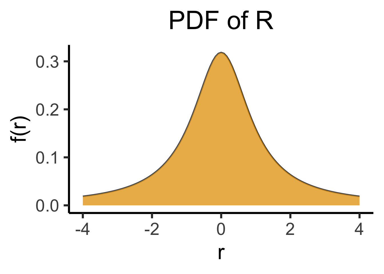
Paxton is a Houston Rockets fan, while Jeff is a Chicago Bulls fan. Paxton creates a RV \(H\) modeling how many games above .500 (wins minus losses) the Rockets will be in a season, while Jeff creates a similar RV \(C\) for the Bulls
They decide to combine their RVs to create a new RV, \(R = \frac{H}{C}\), which now models how much better the Nuggets will be in a season (\(R\) for “Ratio”)
For example, if the Rockets are \(10\) games above .500, while the Bulls are only \(5\) above .500, \(R = \frac{10}{5} = 2\). If they’re both 3 games above .500, \(R = \frac{3}{3} = 1\).

So What’s the Issue?

So far so good. It turns out (though Paxton and Jeff don’t know this) the teams are both mediocre: \(H \sim \mathcal{N}(0,10)\), \(B \sim \mathcal{N}(0,10)\)… What is the distribution of \(R\)?

\[ \begin{gather*} R \sim \text{Cauchy}\left( 0, 1 \right) \end{gather*} \]

\[ \begin{align*} \expect{R} &= ☠️ \\ \Var{R} &= ☠️ \\ M_R(t) &= ☠️ \end{align*} \]

Even worse, this is true regardless of variances: \(D \sim \mathcal{N}(0,d)\) and \(W \sim \mathcal{N}(0,w)\) \(\implies R \sim \text{Cauchy}\left( 0,\frac{d}{w} \right)\)…

Lab 4

Lab 4 Demo

Lab 4 Demo Link
Choose your own adventure:
- Official lab demo
- Math puzzle lab demo
- Move on to Expectation, Variance, Moments

Lab 4 Assignment Prep

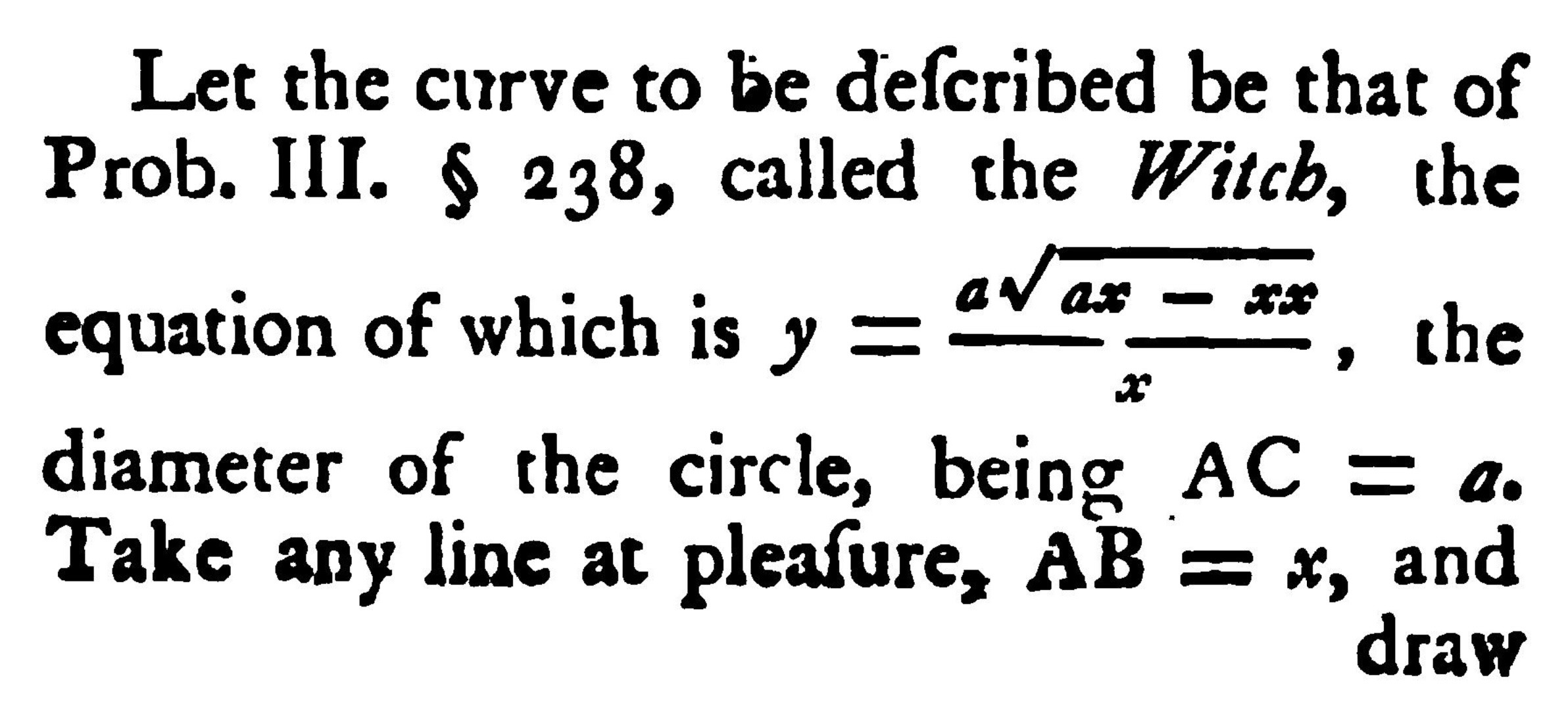
One of my favorite math puzzles ever:

The Problem of the Broken Stick (Gardner 2001, 273–85)

If a stick is broken at random into three pieces, what is the probability that the pieces can be put back together into a triangle?

This cannot be answered without additional information about the exact method of breaking!

One method is to select, independently and at random, two points from the points that range uniformly along the stick, then break the stick at these two points
Suppose, however, that we interpret in a different way the statement “break a stick at random into three pieces”. We break the stick at random, we select randomly one of the two pieces, and we break that piece at random.

Will these two interpretations result in the same probabilities?
If yes, what is that probability?
If no, what are the probabilities in each case?

Lab 4 Assignment

Lab 4 Assignment Link

References

Agnesi, Maria Gaetana. 1801. Analytical Institutions in Four Books: Originally Written in Italian. Taylor and Wilks. https://archive.org/details/analyticalinstit00agnerich/page/n3/mode/2up.

Gardner, Martin. 2001. Colossal Book of Mathematics: Classic Puzzles Paradoxes And Problems. W. W. Norton & Company.

Appendix I: Dirac Delta Function

\(\delta(v)\) from the “Top Secret Fun Fact” slide is called the Dirac Delta function
Enables conversion of discrete distributions into continuous distributions as it represents an “infinite point mass” at \(0\) that can be integrated³:

\[ \delta(v) = \begin{cases}\infty & v = 0 \\ 0 & v \neq 0\end{cases} \]

Its integral also has a name: the Heaviside step function \(\theta(v)\):

\[ \int_{-\infty}^{\infty}\delta(v)dv = \theta(v) = \begin{cases} 1 & v = 0 \\ 0 & v \neq 0\end{cases} \]

Appendix II: Countability of \(\mathbb{Q}\)

Bad definition: “\(\mathbb{N}\) is countable because no \(x \in \mathbb{N}\) between \(0\) and \(1\). \(\mathbb{R}\) is uncountable because infinitely-many \(x \in \mathbb{R}\) between \(0\) and \(1\).” (\(\Rightarrow \mathbb{Q}\) uncountable)
And yet, \(\mathbb{Q}\) is countable…

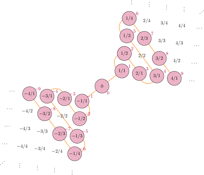
\[ \begin{align*} \begin{array}{ll} s: \mathbb{N} \leftrightarrow \mathbb{Z} & s(n) = (-1)^n \left\lfloor \frac{n+1}{2} \right\rfloor \\ h_+: \mathbb{Z}^+ \leftrightarrow \mathbb{Q}^+ & p_1^{a_1}p_2^{a_2}\cdots \mapsto p_1^{s(a_1)}p_2^{s(a_2)}\cdots \\ h: \mathbb{Z} \leftrightarrow \mathbb{Q} & h(n) = \begin{cases}h_+(n) &n > 0 \\ 0 & n = 0 \\ -h_+(-n) & n < 0\end{cases} \\ (h \circ s): \mathbb{N} \leftrightarrow \mathbb{Q} & ✅🤯 \end{array} \end{align*} \]

Image credit: Rebecca J. Stones, Math StackExchange. Math credit: Thomas Andrews, Math StackExchange

Appendix III: Binomial Triangle

Footnotes

Textbooks sometimes write \(F(x) = \Pr(X \leq x)\), where capital \(X\) is a RV while lowercase \(x\) is a particular value, like \(3\). To reduce confusion, I use \(X\) for the RV and \(v\) for the value at which we’re checking the CDF. Also note capitalized CDF but lowercase pmf/pdf, matching mathematical notation: \(f_X(v)\) is the derivative of \(F_X(v)\).↩︎
Fun way to avoid memorizing! Imagine a pyramid like \(\genfrac{}{}{0pt}{}{}{\boxed{\phantom{1}}}\genfrac{}{}{0pt}{}{\boxed{\phantom{1}}}{}\genfrac{}{}{0pt}{}{}{\boxed{\phantom{1}}}\), where boxes are slots for numbers. Put a \(1\) in box at the top. In bottom row, fill each slot with the sum of the two numbers above-left and above-right of it. Since \(1 + \text{(nothing)} = 1\), this looks like: \(\genfrac{}{}{0pt}{}{}{1}\genfrac{}{}{0pt}{}{1}{}\genfrac{}{}{0pt}{}{}{1}\). Continue filling in rows this way, so next row looks like \(\genfrac{}{}{0pt}{}{}{1}\genfrac{}{}{0pt}{}{1}{}\genfrac{}{}{0pt}{}{}{2}\genfrac{}{}{0pt}{}{1}{}\genfrac{}{}{0pt}{}{}{1}\), then \(\genfrac{}{}{0pt}{}{}{1}\genfrac{}{}{0pt}{}{1}{}\genfrac{}{}{0pt}{}{}{3}\genfrac{}{}{0pt}{}{2}{}\genfrac{}{}{0pt}{}{}{3}\genfrac{}{}{0pt}{}{1}{}\genfrac{}{}{0pt}{}{}{1}\), etc. The \(k\)th number in the \(N\)th row (counting from \(0\)) is \(\binom{N}{k}\). Appendix shows triangle written out to 7th row!↩︎
This is leaving out some of the complexities of defining this function so it “works” in this way: for example, we need to use the Lebesgue integral rather than the (standard) Riemann integral for it to be defined at all, and even then it technically fails the conditions necessary for a fully-well-defined Lebesgue integral. For full details see this section from the Wiki article on PDFs, and follow the links therein.↩︎