Week 4: Continuous Distributions
DSAN 5100: Probabilistic Modeling and Statistical Computing
Section 01
Tuesday, September 16, 2025
Discrete vs. Continuous
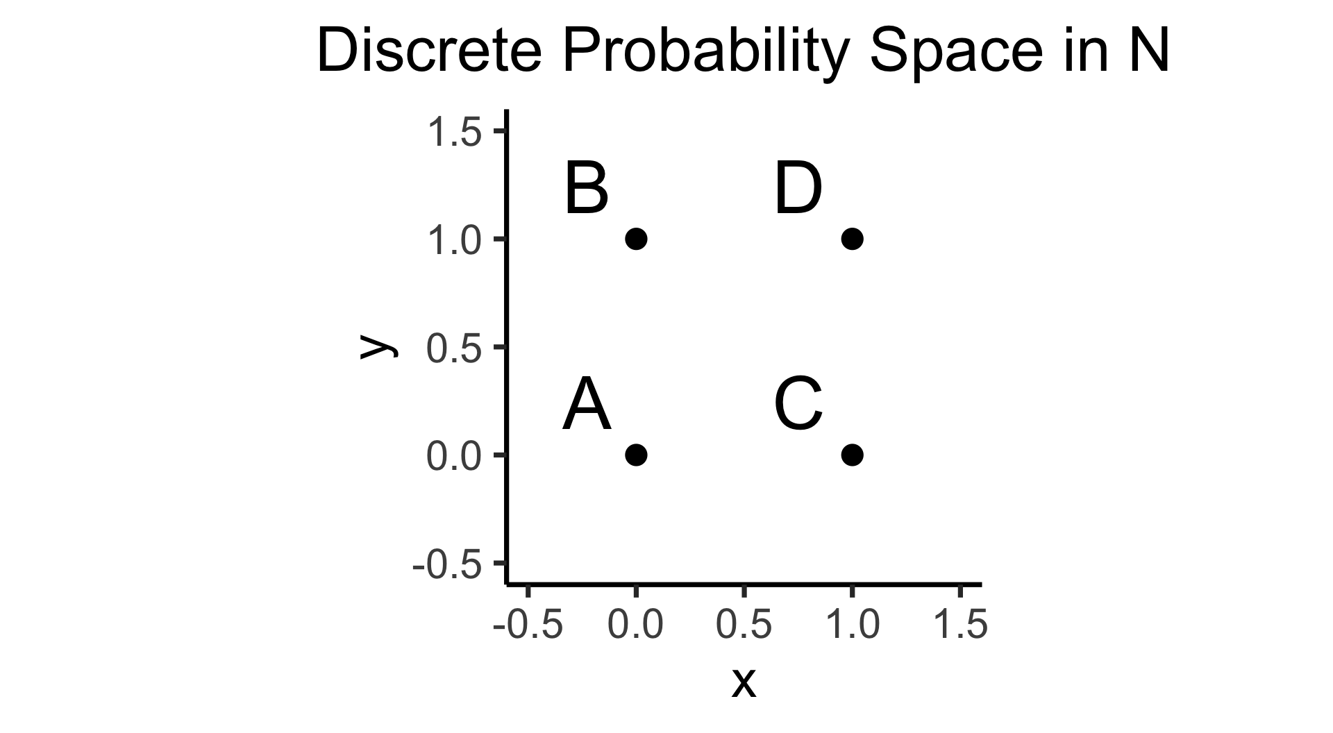
- Discrete = “Easy mode”: Based (intuitively) on sets
- \(\Pr(A)\): Four equally-likely marbles \(\{A, B, C, D\}\) in box, what is probability I pull out \(A\)?
\[ \Pr(A) = \underset{\mathclap{\small \text{Probability }\textbf{mass}}}{\boxed{\frac{|\{A\}|}{|\Omega|}}} = \frac{1}{|\{A,B,C,D\}|} = \frac{1}{4} \]
- Continuous = “Hard mode”: Based (intuitively) on areas
- \(\Pr(A)\): Throw dart at random point in square, what is probability I hit \(\require{enclose}\enclose{circle}{\textsf{A}}\)?
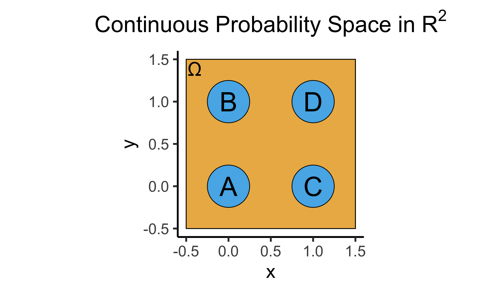
\[ \Pr(A) = \underset{\mathclap{\small \text{Probability }\textbf{density}}}{\boxed{\frac{\text{Area}(\{A\})}{\text{Area}(\Omega)}}} = \frac{\pi r^2}{s^2} = \frac{\pi \left(\frac{1}{4}\right)^2}{4} = \frac{\pi}{64} \]
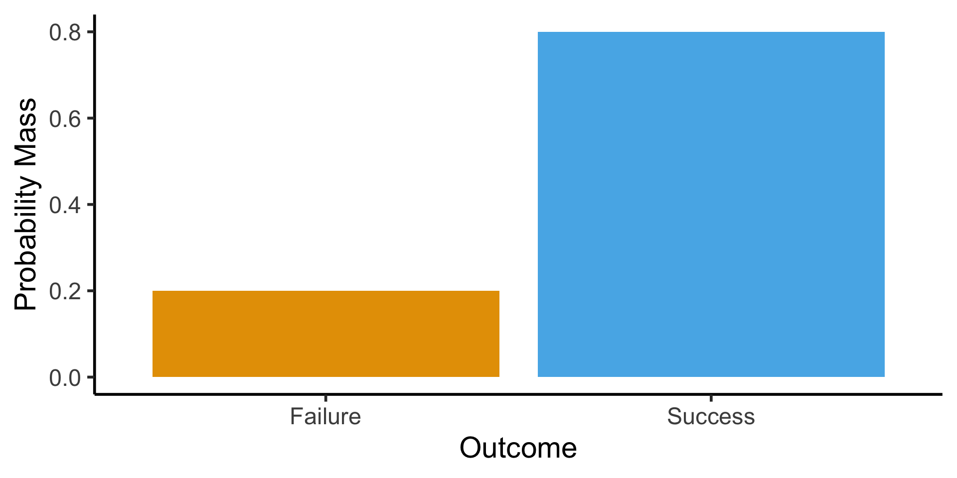
Bernoulli Distribution
- Single trial with two outcomes, “success” (1) or “failure” (0): basic model of a coin flip (heads = 1, tails = 0)
- \(X \sim \text{Bern}({\color{purple} p}) \implies \mathcal{R}_X = \{0,1\}, \; \Pr(X = 1) = {\color{purple}p}\).
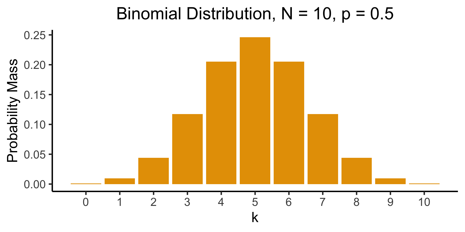
Visualizing the Binomial

Geometric Distribution
- Likelihood that we need \({\color{purple}k}\) trials to get our first success. \(X \sim \text{Geom}({\color{purple}k},{\color{purple}p}) \implies \mathcal{R}_X = \{1, 2, \ldots\}\)
- \(\Pr(X = k) = \underbrace{(1-p)^{k-1}}_{\small k - 1\text{ failures}}\cdot \underbrace{p}_{\mathclap{\small \text{success}}}\)
- Probability of \(k\) trials before first success

[Recall] Binomial Distribution
The Emergence of Order
- Who can guess the state of this process after 10 steps, with 1 person?
- 10 people? 50? 100? (If they find themselves on the same spot, they stand on each other’s heads)
- 100 steps? 1000?

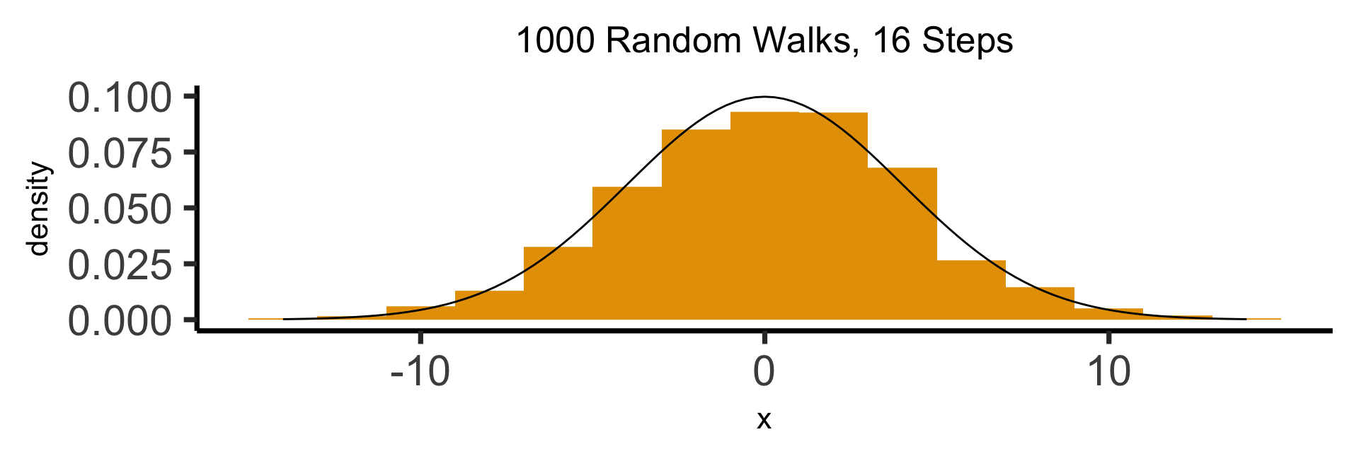
The Result: 16 Steps

The Result: 64 Steps
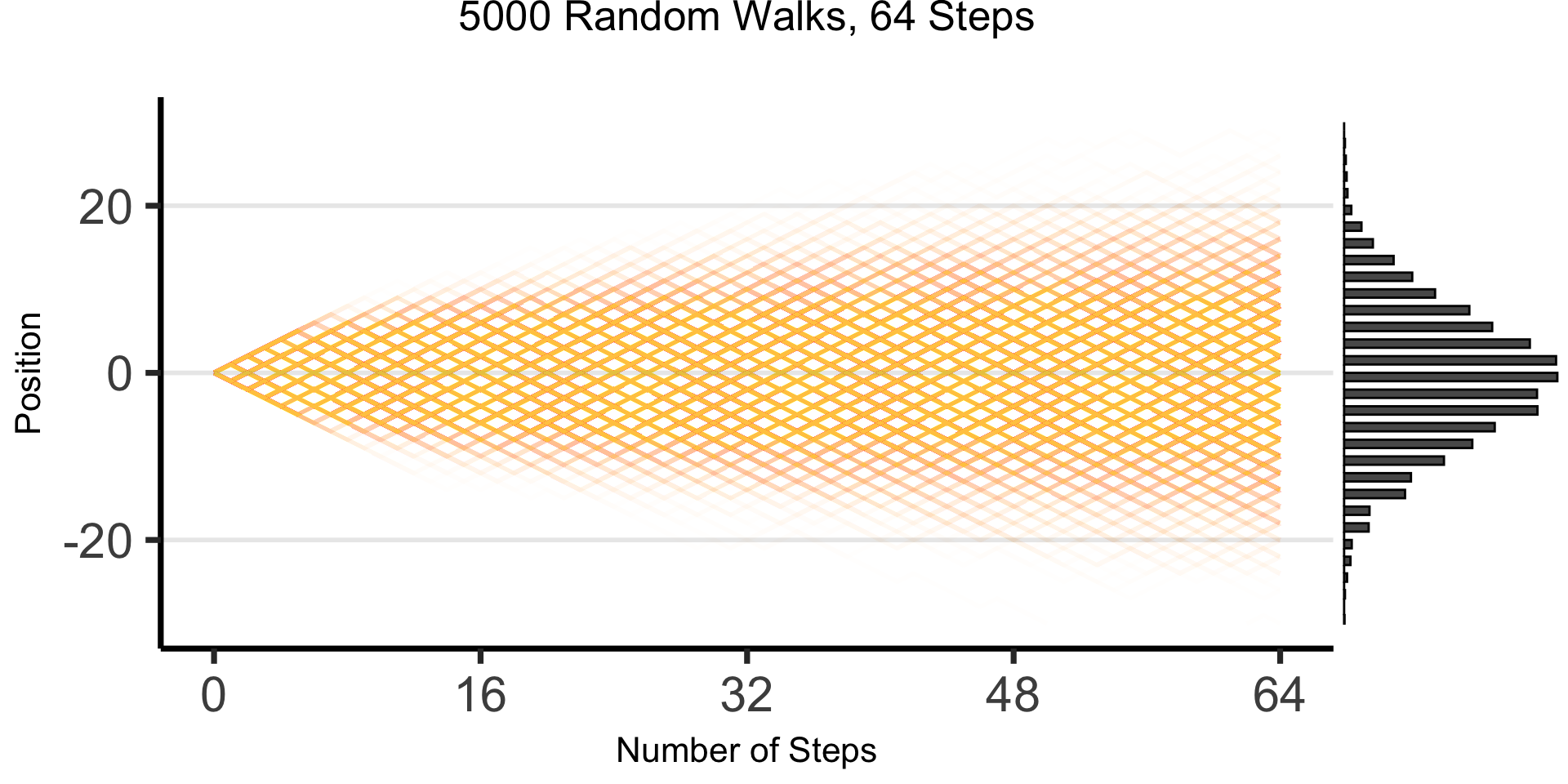

What’s Going On Here?

(Stay tuned for Markov processes \(\overset{t \rightarrow \infty}{\leadsto}\) Stationary distributions!)
[Recall] Discrete Uniform Distribution
Code
library(tibble)
bar_data <- tribble(
  ~x, ~prob,
  1, 1/6,
  2, 1/6,
  3, 1/6,
  4, 1/6,
  5, 1/6,
  6, 1/6
)
ggplot(bar_data, aes(x=x, y=prob)) +
  geom_bar(stat="identity", fill=cbPalette[1]) +
  labs(
    title="Discrete Uniform pmf: a = 1, b = 6",
    y="Probability Mass",
    x="Value"
  ) +
  scale_x_continuous(breaks=seq(1,6)) +
  dsan_theme("half")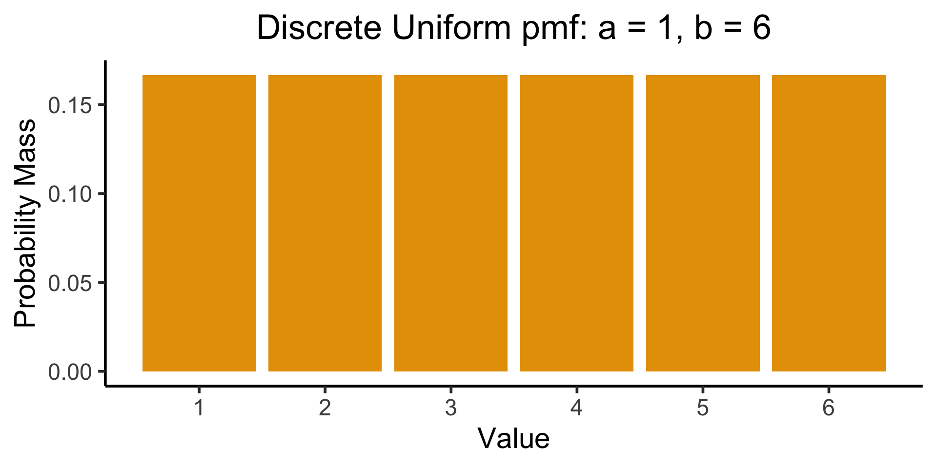
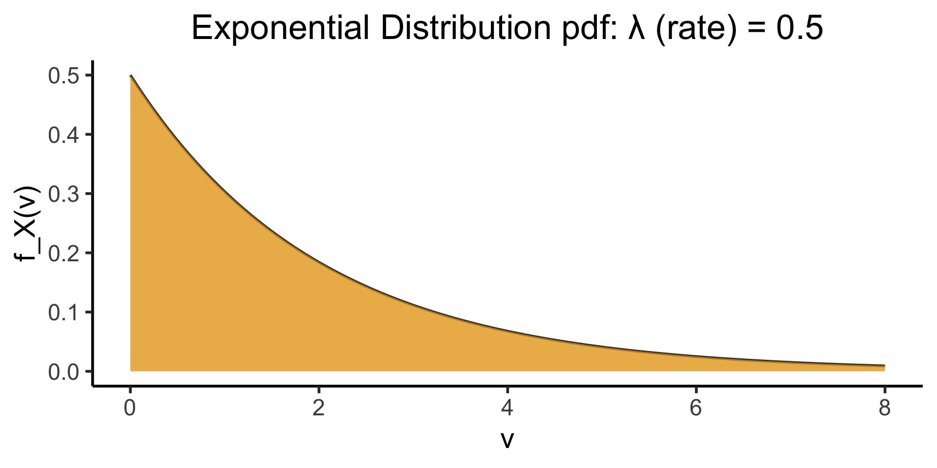
Exponential Distribution
- Recall the (discrete) Geometric Distribution:
Code
library(ggplot2)
k <- seq(0, 8)
prob <- dgeom(k, 0.5)
bar_data <- tibble(k, prob)
ggplot(bar_data, aes(x = k, y = prob)) +
    geom_bar(stat = "identity", fill = cbPalette[1]) +
    labs(
        title = "Geometric Distribution pmf: p = 0.5",
        y = "Probability Mass"
    ) +
    scale_x_continuous(breaks = seq(0, 8)) +
    dsan_theme("half")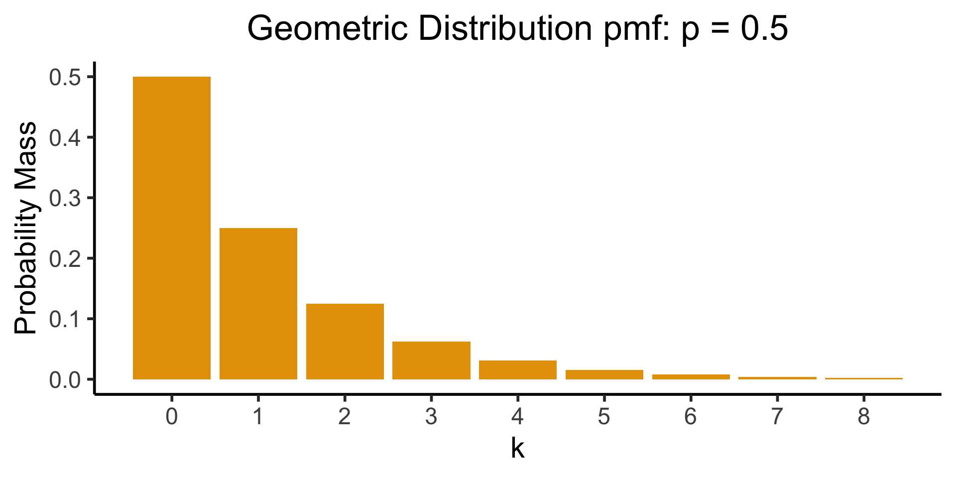
Now In Continuous Form!
Code
my_dexp <- function(x) dexp(x, rate = 1/2)
ggplot(data.frame(x=c(0,8)), aes(x=x)) +
  stat_function(fun=my_dexp, size=g_linesize, fill=cbPalette[1], alpha=0.8) +
  stat_function(fun=my_dexp, geom='area', fill=cbPalette[1], alpha=0.75) +
  dsan_theme("half") +
  labs(
    title="Exponential Distribution pdf: λ (rate) = 0.5",
    x = "v",
    y = "f_X(v)"
  )
The Dreaded Cauchy Distribution
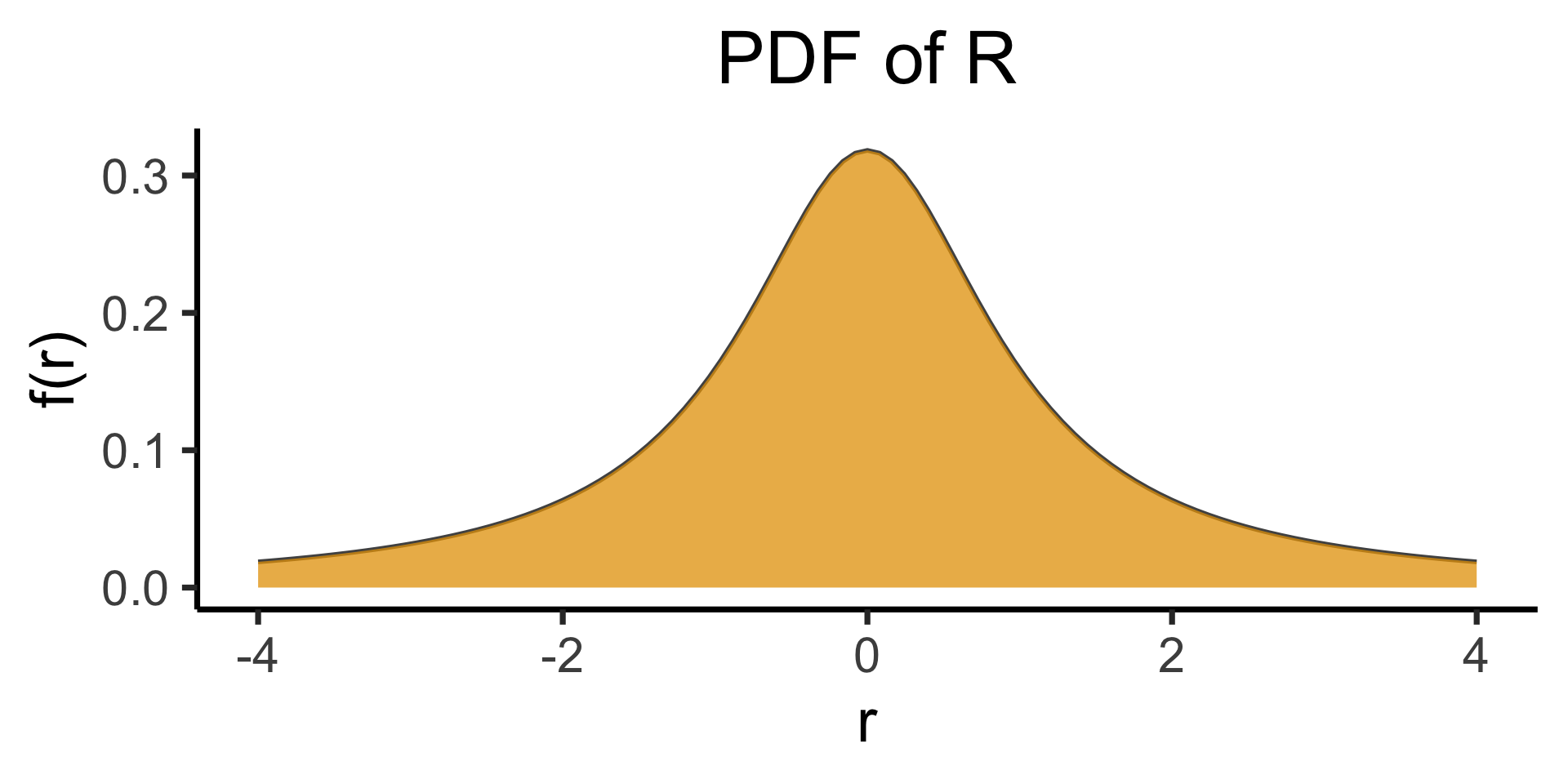
- Paxton is a Houston Rockets fan, while Jeff is a Chicago Bulls fan. Paxton creates a RV \(H\) modeling how many games above .500 (wins minus losses) the Rockets will be in a season, while Jeff creates a similar RV \(C\) for the Bulls
- They decide to combine their RVs to create a new RV, \(R = \frac{H}{C}\), which now models how much better the Nuggets will be in a season (\(R\) for “Ratio”)
- For example, if the Rockets are \(10\) games above .500, while the Bulls are only \(5\) above .500, \(R = \frac{10}{5} = 2\). If they’re both 3 games above .500, \(R = \frac{3}{3} = 1\).
So What’s the Issue?
So far so good. It turns out (though Paxton and Jeff don’t know this) the teams are both mediocre: \(H \sim \mathcal{N}(0,10)\), \(B \sim \mathcal{N}(0,10)\)… What is the distribution of \(R\)?
\[ \begin{gather*} R \sim \text{Cauchy}\left( 0, 1 \right) \end{gather*} \]
\[ \begin{align*} \expect{R} &= ☠️ \\ \Var{R} &= ☠️ \\ M_R(t) &= ☠️ \end{align*} \]
Even worse, this is true regardless of variances: \(D \sim \mathcal{N}(0,d)\) and \(W \sim \mathcal{N}(0,w)\) \(\implies R \sim \text{Cauchy}\left( 0,\frac{d}{w} \right)\)…
Appendix II: Countability of \(\mathbb{Q}\)
- Bad definition: “\(\mathbb{N}\) is countable because no \(x \in \mathbb{N}\) between \(0\) and \(1\). \(\mathbb{R}\) is uncountable because infinitely-many \(x \in \mathbb{R}\) between \(0\) and \(1\).” (\(\Rightarrow \mathbb{Q}\) uncountable)
- And yet, \(\mathbb{Q}\) is countable…
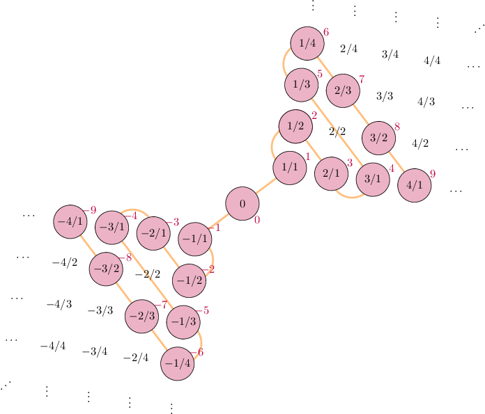
\[ \begin{align*} \begin{array}{ll} s: \mathbb{N} \leftrightarrow \mathbb{Z} & s(n) = (-1)^n \left\lfloor \frac{n+1}{2} \right\rfloor \\ h_+: \mathbb{Z}^+ \leftrightarrow \mathbb{Q}^+ & p_1^{a_1}p_2^{a_2}\cdots \mapsto p_1^{s(a_1)}p_2^{s(a_2)}\cdots \\ h: \mathbb{Z} \leftrightarrow \mathbb{Q} & h(n) = \begin{cases}h_+(n) &n > 0 \\ 0 & n = 0 \\ -h_+(-n) & n < 0\end{cases} \\ (h \circ s): \mathbb{N} \leftrightarrow \mathbb{Q} & ✅🤯 \end{array} \end{align*} \]
Appendix III: Binomial Triangle
