Week 2B: Random Variables

DSAN 5100: Probabilistic Modeling and Statistical Computing
Section 01

Class Sessions

Author

Purna Gamage, Amineh Zadbood, and Jeff Jacobs

Published

Tuesday, September 2, 2025

Open slides in new window →

Probability Fundamentals

Logic, Sets, and Probability

Deep connection between objects and operations of logic, set theory, and probability:

	Logic	Set Theory	Probability Theory
Objects	Predicates \(p, q \in \{T, F\}\)	Sets \(S = \{a, b, \ldots\}\)	Events \(E = \{TT, TH, HT, HH\}\)
Conjunction	And (\(\wedge\)) \(p \wedge q\)	Intersection (\(\cap\)) \(A \cap B\)	Multiplication (\(\times\)): \(\Pr(E_1 \cap E_2) = \Pr(E_1)\times \Pr(E_2)\)
Disjunction	Or (\(\vee\)) \(p \vee q\)	Union (\(\cup\)) \(A \cup B\)	Addition (\(+\)): \(\Pr(E_1 \cup E_2) =\) \(\Pr(E_1) + \Pr(E_2) - \Pr(E_1 \wedge E_2)\)
Negation	Not (\(\neg\)) \(\neg p\)	Complement (\(^c\)) \(S^c\)	Subtract from 1 \(\Pr(A^c) = 1 - \Pr(A)\)

Example: Flipping Two Coins

Logic: We can define 4 predicates:
- \(p_1\) = “First result is \(H\)”, \(q_1\) = “First result is \(T\)”
- \(p_2\) = “Second result is \(H\)”, \(q_2\) = “Second result is \(T\)”
Logical formulas:
- \(f_1 = p_1 \wedge q_2\): “First result is \(H\) and second result is \(T\)”
- \(f_2 = p_1 \vee q_2\): “First result is \(H\) or second result is \(T\)”
- \(f_3 = \neg p_1\): “First result is not \(H\)”
The issue?: We don’t know, until after the coins have been flipped, whether these are true or false!
But, we should still be able to say something about their likelihood, for example, whether \(f_1\) or \(f_2\) is more likely to happen… Enter probability theory!

Logic \(\rightarrow\) Probability

Probability theory lets us reason about the uncertainty surrounding logical predicates like \(p\) and \(q\), by:
1. encoding them as sets of possibilities \(P\) and \(Q\), and
2. representing uncertainty around a given possibility using a probability measure \(\Pr: S \mapsto [0,1]\),
thus allowing us to reason about
1. the likelihood of these set-encoded predicates on their own: \(\Pr(P)\) and \(\Pr(Q)\), but also
2. their logical connections: \(\Pr(p \wedge q) = \Pr(P \cap Q)\), \(\Pr(\neg p) = \Pr(P^c)\), and so on.

Flipping Two Coins: Logic \(\rightarrow\) Probability

Returning to the two coins example: we can look at the predicates and see that they exhaust all possibilities, so that we can define a sample space \(\Omega = \{TT, TH, HT, HH\}\) of all possible outcomes of our coin-flipping experiment, noting that \(|\Omega| = 4\), so there are 4 possible outcomes.
Then we can associate each predicate with an event, a subset of the sample space, and use our naïve definition to compute the probability of these events:

Predicate	Event	Probability
\(p_1\) = “First result is \(H\)”	\(P_1 = \{HT, HH\}\)	\(\Pr(P_1) = \frac{\|P_1\|}{\|\Omega\|} = \frac{2}{4} = \frac{1}{2}\)
\(q_1\) = “First result is \(T\)”	\(Q_1 = \{TT, TH\}\)	\(\Pr(Q_1) = \frac{\|Q_1\|}{\|\Omega\|} = \frac{2}{4} = \frac{1}{2}\)
\(p_2\) = “Second result is \(H\)”	\(P_2 = \{TH, HH\}\)	\(\Pr(P_2) = \frac{\|P_2\|}{\|\Omega\|} = \frac{2}{4} = \frac{1}{2}\)
\(q_2\) = “Second result is \(T\)”	\(Q_2 = \{TT, HT\}\)	\(\Pr(Q_2) = \frac{\|Q_2\|}{\|\Omega\|} = \frac{2}{4} = \frac{1}{2}\)

Moving from Predicates to Formulas

Notice that, in the four rows of the previous table, we were only computing the probabilities of “simple” events: events corresponding to a single predicate
But we promised that probability theory lets us compute probabilities for logical formulas as well! …The magic of encoding events as sets becomes clear:

Formula	Event	Probability
\(f_1 = p_1 \wedge q_2\)	\[ \begin{align} F_1 &= P_1 \cap Q_2 \\ &= \{HT, HH\} \cap \{TT, HT\} \\ &= \{HT\} \end{align} \]	\[\begin{align} \Pr(F_1) &= \Pr(\{HT\}) \\ &= \frac{\|\{HT\}\|}{\|S\|} = \frac{1}{4} \phantom{= \frac{1}{4} = \frac{1}{4}} \end{align}\]
\(f_2 = p_1 \vee q_2\)	\[\begin{align} F_2 &= P_1 \cup Q_2 \\ &= \{HT, HH\} \cup \{TT, HT\} \\ &= \{TT, HT, HH\} \end{align}\]	\[\begin{align} \Pr(F_2) &= \Pr(\{TT, HT, HH\}) \\ &= \frac{\|\{TT, HT, HH\}\|}{\|S\|} = \frac{3}{4} \end{align}\]
\(f_3 = \neg p_1\)	\[\begin{align} F_3 &= P_1^c \\ &= \{HT, HH\}^c \phantom{\cup \{TT, HT\}} \\ &= \{TT, TH\}\end{align}\]	\[\begin{align} \Pr(F_3) &= \Pr(\{TT, TH\}) \\ &= \frac{\|\{TT, TH\}\|}{\|S\|} = \frac{2}{4} = \frac{1}{2} \end{align}\]

Using “Rules” of Probability

Hopefully, you found all this churning through set theory to be tedious… ☠️
This is where rules of probability come from! They simplify set-theoretic computations into simple multiplications, additions, and subtractions:
- \(\Pr(A \cap B) = \Pr(A) \times \Pr(B)\)
- \(\Pr(A \cup B) = \Pr(A) + \Pr(B) - \Pr(A \cap B)\)
- \(\Pr(A^c) = 1 - \Pr(A)\)
Since we know probabilities of the “simple” events \(P_1\), \(Q_1\), \(P_2\), \(Q_2\), we don’t need to “look inside them”! Just take the probabilities and multiply/add/subtract as needed:

Formula	Event	Probability
\(f_1 = p_1 \wedge q_2\)	\(F_1 = P_1 \cap Q_2\)	\(\Pr(F_1) = \Pr(P_1) \times \Pr(Q_2) = \frac{1}{2}\times \frac{1}{2} = \frac{1}{4}\)
\(f_2 = p_1 \vee q_2\)	\(F_2 = P_1 \cup Q_2\)	\[\textstyle{\begin{align} \textstyle \Pr(F_2) &= \Pr(P_1) + \Pr(Q_2) - \Pr(P_1 \cap Q_2) \\ \textstyle &= \frac{1}{2} + \frac{1}{2} - \frac{1}{4} = \frac{3}{4} \end{align}}\]
\(f_3 = \neg p_1\)	\(F_3 = P_1^c\)	\(\Pr(F_3) = 1 - \Pr(P_1) = 1 - \frac{1}{2} = \frac{1}{2}\)

“Importing” Results from Logic

This deep connection between the three fields means that, if we have some useful theorem or formula from one field, we can immediately put it to use in another!
For example: DeMorgan’s Laws were developed in logic (DeMorgan was a 19th-century logician), and basically just tell us how to distribute logic operators:

\[ \begin{align*} \underbrace{\neg(p \wedge q)}_{\text{``}p\text{ and }q\text{'' is not true}} &\iff \underbrace{\neg p \vee \neg q}_{p\text{ is not true or }q\text{ is not true}} \\ \underbrace{\neg(p \vee q)}_{\text{``}p\text{ or }q\text{'' is not true}} &\iff \underbrace{\neg p \wedge \neg q}_{p\text{ is not true and }q\text{ is not true}} \end{align*} \]

Converting to Probability Theory

So, using the same principles we used in our coin flipping examples, we can consider events \(P\) and \(Q\), and get the following “translation” of DeMorgan’s Laws:

Logic	Set Theory	Probability Theory
\(\neg(p \wedge q) = \neg p \vee \neg q\)	\((P \cap Q)^c = P^c \cup Q^c\)	\(\Pr((P \cap Q)^c) = \Pr(P^c \cup Q^c)\)
\(\neg(p \vee q) = \neg p \wedge \neg q\)	\((P \cup Q)^c = P^c \cap Q^c\)	\(\Pr((P \cup Q)^c) = \Pr(P^c \cap Q^c)\)

Note that, since these are isomorphic to one another, we could have derived DeMorgan’s Laws from within probability theory, rather than the other way around:

\[ \begin{align*} \Pr((P \cap Q)^c) &= 1 - \Pr(P \cap Q) = 1 - \Pr(P)\Pr(Q) \\ &= 1 - (1-\Pr(P^c))(1 - \Pr(Q^c)) \\ &= 1 - [1 - \Pr(P^c) - \Pr(Q^c) + \Pr(P^c)\Pr(Q^c)] \\ &= \Pr(P^c) + \Pr(Q^c) - \Pr(P^c)\Pr(Q^c) \\ &= \Pr(P^c) + \Pr(Q^c) - \Pr(P^c \cap Q^c) \\ &= \Pr(P^c \cup Q^c) \; ✅ \end{align*} \]

Univariate Statistics

Random Variables

Recall our discussion of random variables: used by analogy to algebra, since we can do math with them:
Just as \(2 \cdot 3\) is shorthand for \(2 + 2 + 2\), can define \(X\) as shorthand for possible outcomes of random process:

\[ \begin{align*} S = \{ &\text{result of dice roll is 1}, \\ &\text{result of dice roll is 2}, \\ &\text{result of dice roll is 3}, \\ &\text{result of dice roll is 4}, \\ &\text{result of dice roll is 5}, \\ &\text{result of dice roll is 6}\} \rightsquigarrow X \in \{1,\ldots,6\} \end{align*} \]

Random Variables as Events

Each value \(v_X\) that a random variable \(X\) can take on gives rise to an event \(X = v_X\): the event that the random variable \(X\) takes on value \(v\).
Since \(X = v_X\) is an event, we can compute its probability \(\Pr(X = v_X)\)!

Event in words	Event in terms of RV
Result of dice roll is 1	\(X = 1\)
Result of dice roll is 2	\(X = 2\)
Result of dice roll is 3	\(X = 3\)
Result of dice roll is 4	\(X = 4\)
Result of dice roll is 5	\(X = 5\)
Result of dice roll is 6	\(X = 6\)

Doing Math with Events

We’ve seen how \(\Pr()\) “encodes” logical expressions involving uncertain outcomes.
Even more powerful when paired with the notion of random variables: lets us also “encode” mathematical expressions involving uncertain quantities!
Consider an experiment where we roll two dice. Let \(X\) be the RV encoding the outcome of the first roll, and \(Y\) be the RV encoding the outcome of the second roll.
We can compute probabilities involving \(X\) and \(Y\) separately, e.g., \(\Pr(X = 1) = \frac{1}{6}\), but we can also reason probabilistically about mathematical expressions involving \(X\) and \(Y\)! For example, we can reason about their sum:

\[ \begin{align*} \Pr(\text{rolls sum to 10}) &= \Pr(X + Y = 10) \\ &= \Pr(Y = 10 - X) \end{align*} \]

Or about how the outcome of one roll will relate to the outcome of the other:

\[ \begin{align*} \Pr(\text{first roll above mean}) &= \Pr\left(X > \frac{X+Y}{2}\right) \\ &= \Pr(2X > X+Y) = \Pr(X > Y) \end{align*} \]

Are Random Variables All-Powerful??

Just remember that probability \(\Pr(\cdot)\) is always probability of an event—random variables are just shorthand for quantifiable events.
Not all events can be simplified via random variables!
- \(\text{catch a fish} \mapsto \Pr(\text{trout}), \Pr(\text{bass}), \ldots\)
What types of events can be quantified like this?
- (Hint: It has to do with a key topic in the early weeks of both DSAN 5000 and 5100…)

The answer is, broadly, any situation where you’re modeling things, like dice rolls, where mathematical operations like addition, multiplication, etc. make sense. So, if we’re modeling dice, it makes sense to say e.g. “result is 6” + “result is 3” = “total is 9”. More on the next page!

Recall: Types of Variables

Categorical
- No meaningful way to order values: \(\{\text{trout}, \text{bass}, \ldots \}\)
Ordinal
- Can place in order (bigger, smaller), though gaps aren’t meaningful: \(\{{\color{orange}\text{great}},{\color{orange}\text{greater}},{\color{orange}\text{greatest}}\}\)
- \({\color{orange}\text{greater}} \overset{?}{=} 2\cdot {\color{orange}\text{great}} - 1\)
Cardinal
- Can place in order, and gaps are meaningful \(\implies\) can do “standard” math with them! Example: \(\{{\color{blue}1},{\color{blue}2},\ldots,{\color{blue}10}\}\)
- \({\color{blue}7} \overset{\text{~✅~}}{=} 2 \cdot {\color{blue}4} - 1\)
- If events have this structure (meaningful way to define multiplication, addition, subtraction), then we can analyze them as random variables

Visualizing Discrete RVs

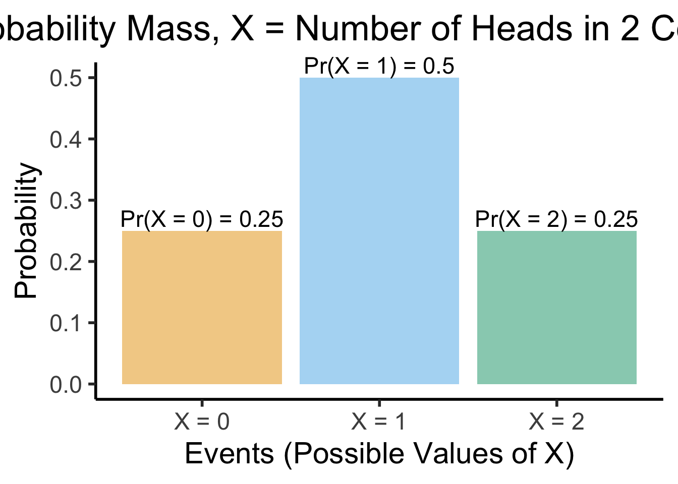
Ultimate Probability Pro-Tip: When you hear “discrete distribution”, think of a bar graph: \(x\)-axis = events, bar height = probability of events
Two coins example: \(X\) = RV representing number of heads obtained in two coin flips

(Preview:) Visualizing Continuous RVs

This works even for continuous distributions, if you focus on the area under the curve instead of the height:

funcShaded <- function(x, lower_bound, upper_bound) {
    y <- dnorm(x)
    y[x < lower_bound | x > upper_bound] <- NA
    return(y)
}
funcShadedBound1 <- function(x) funcShaded(x, -Inf, 0)
funcShadedBound2 <- function(x) funcShaded(x, 0.2, 1.8)
funcShadedBound3 <- function(x) funcShaded(x, 2, Inf)

norm_plot <- ggplot(data.frame(x=c(-3,3)), aes(x = x)) +
    stat_function(fun = dnorm) +
    labs(
      title="Probability Density, X Normally Distributed",
      x="Possible Values of X",
      y="Probability Density"
    ) +
    dsan_theme("half") +
    theme(legend.position = "none") +
    coord_cartesian(clip = "off")
label_df <- tribble(
  ~x, ~y, ~label,
  -0.8, 0.1, "Pr(X < 0) = 0.5",
  1.0, 0.05, "Pr(0.2 < X < 1.8)\n= 0.385",
  2.5,0.1,"Pr(X > 1.96)\n= 0.025"
)
shaded_plot <- norm_plot +
  stat_function(fun = funcShadedBound1, geom = "area", fill=cbPalette[1], alpha = 0.5) +
  stat_function(fun = funcShadedBound2, geom = "area", fill=cbPalette[2], alpha = 0.5) +
  stat_function(fun = funcShadedBound3, geom = "area", fill=cbPalette[3], alpha = 0.5) +
  geom_text(label_df, mapping=aes(x = x, y = y, label = label), size=6)
shaded_plot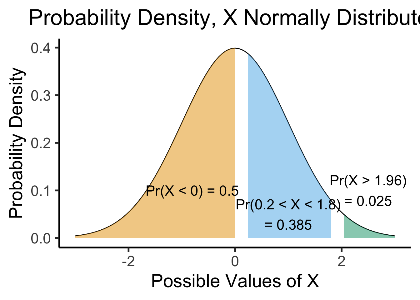

Probability Theory Gives Us Distributions for RVs, not Numbers!

We’re going beyond “base” probability theory if we want to summarize these distributions
However, we can understand a lot about the full distribution by looking at some basic summary statistics. Most common way to summarize:

\(\underbrace{\text{point estimate}}_{\text{mean/median}}\)

\(\pm\)

\(\underbrace{\text{uncertainty}}_{\text{variance/standard deviation}}\)

Example: Game Reviews

library(readr)
fig_title <- "Reviews for a Popular Nintendo Switch Game"
#score_df <- read_csv("https://gist.githubusercontent.com/jpowerj/8b2b6a50cef5a682db640e874a14646b/raw/bbe07891a90874d1fe624224c1b82212b1ac8378/totk_scores.csv")
score_df <- read_csv("https://gist.githubusercontent.com/jpowerj/8b2b6a50cef5a682db640e874a14646b/raw/e3c2b9d258380e817289fbb64f91ba9ed4357d62/totk_scores.csv")
mean_score <- mean(score_df$score)
library(ggplot2)
ggplot(score_df, aes(x=score)) +
  geom_histogram() +
  #geom_vline(xintercept=mean_score) +
  labs(
    title=fig_title,
    x="Review Score",
    y="Number of Reviews"
  ) +
  dsan_theme("full")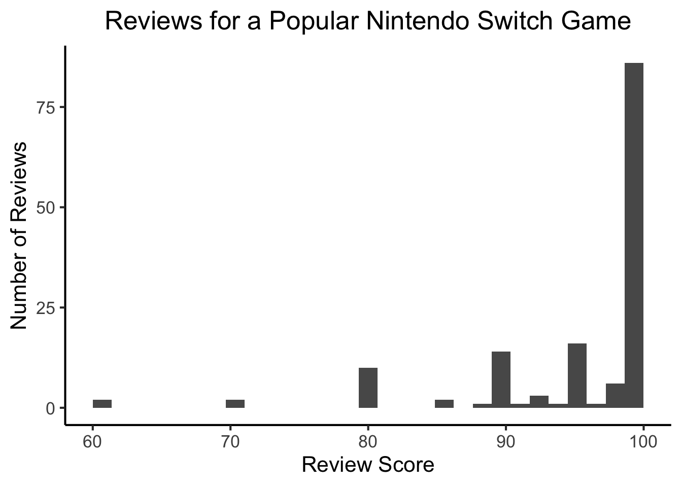

Adding a Single Line

library(readr)
mean_score <- mean(score_df$score)
mean_score_label <- sprintf("%0.2f", mean_score)
library(ggplot2)
ggplot(score_df, aes(x=score)) +
  geom_histogram() +
  geom_vline(aes(xintercept=mean_score, linetype="dashed"), color="purple", size=1) +
  scale_linetype_manual("", values=c("dashed"="dashed"), labels=c("dashed"="Mean Score")) +
  # Add single additional tick
  scale_x_continuous(breaks=c(60, 70, 80, 90, mean_score, 100), labels=c("60","70","80","90",mean_score_label,"100")) +
  labs(
    title=fig_title,
    x="Review Score",
    y="Number of Reviews"
  ) +
  dsan_theme("full") +
  theme(
    legend.title = element_blank(),
    legend.spacing.y = unit(0, "mm")
  ) +
  theme(axis.text.x = element_text(colour = c('black', 'black','black', 'black', 'purple', 'black')))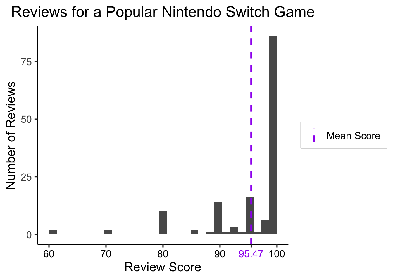

Or a Single Ribbon

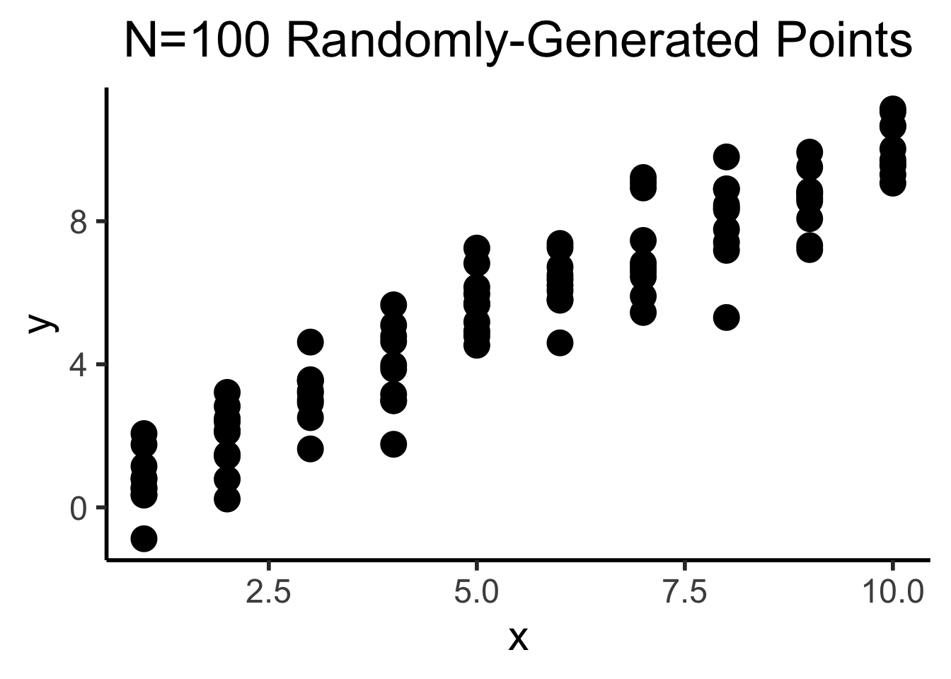
library(tibble)
N <- 10
# Each x value gets 10 y values
x <- sort(rep(seq(1,10),10))
y <- x + rnorm(length(x), 0, 5)
df <- tibble(x=x,y=y)
total_N <- nrow(df)
ggplot(df, aes(x=x,y=y)) +
  geom_point(size=g_pointsize) +
  dsan_theme("column") +
  labs(
    title=paste0("N=",total_N," Randomly-Generated Points")
  )
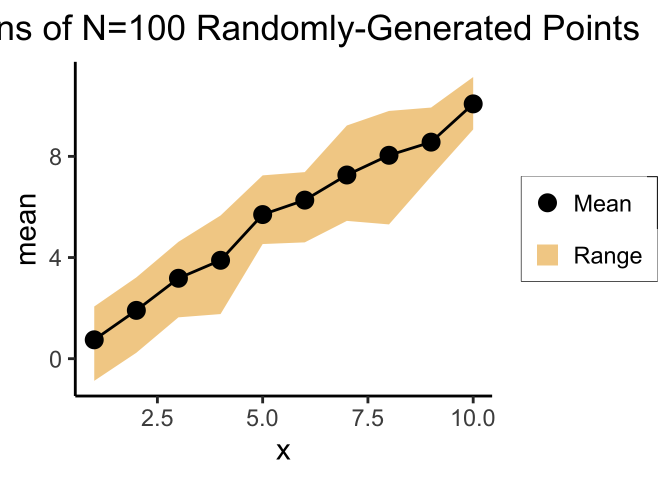
# This time, just the means
library(dplyr)
mean_df <- df %>% group_by(x) %>% summarize(mean=mean(y), min=min(y), max=max(y))
ggplot(mean_df, aes(x=x, y=mean)) +
  geom_ribbon(aes(ymin=min, ymax=max, fill="ribbon"), alpha=0.5) +
  geom_point(aes(color="mean"), size=g_pointsize) +
  geom_line(size=g_linesize) +
  dsan_theme("half") +
  scale_color_manual("", values=c("mean"="black"), labels=c("mean"="Mean")) +
  scale_fill_manual("", values=c("ribbon"=cbPalette[1]), labels=c("ribbon"="Range")) +
  remove_legend_title() +
  labs(
    title=paste0("Means of N=",total_N," Randomly-Generated Points")
  )
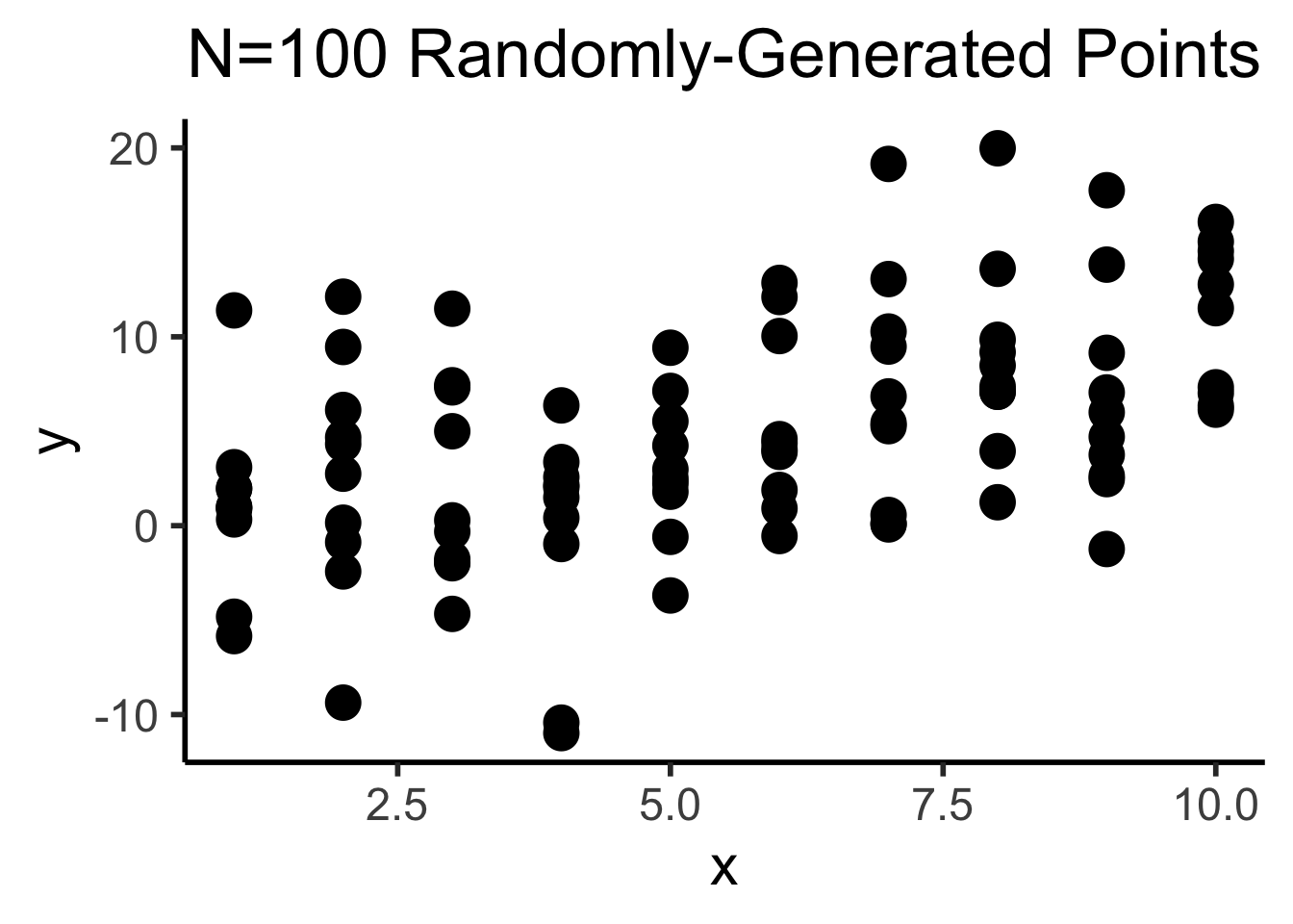
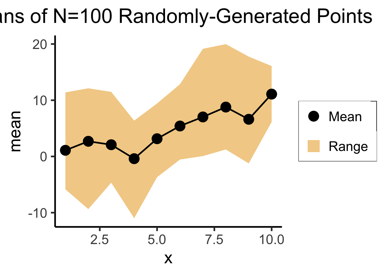
library(tibble)
N <- 100
# Each x value gets 10 y values
x <- sort(rep(seq(1,10),10))
y <- x + rnorm(length(x), 0, 1)
df <- tibble(x=x,y=y)
total_N <- nrow(df)
ggplot(df, aes(x=x,y=y)) +
  geom_point(size=g_pointsize) +
  dsan_theme("column") +
  labs(
    title=paste0("N=",total_N," Randomly-Generated Points")
  )
# This time, just the means
library(dplyr)
mean_df <- df %>% group_by(x) %>% summarize(mean=mean(y), min=min(y), max=max(y))
ggplot(mean_df, aes(x=x, y=mean)) +
  geom_ribbon(aes(ymin=min, ymax=max, fill="ribbon"), alpha=0.5) +
  geom_point(aes(color="mean"), size=g_pointsize) +
  geom_line(size=g_linesize) +
  dsan_theme("half") +
  scale_color_manual("", values=c("mean"="black"), labels=c("mean"="Mean")) +
  scale_fill_manual("", values=c("ribbon"=cbPalette[1]), labels=c("ribbon"="Range")) +
  remove_legend_title() +
  labs(
    title=paste0("Means of N=",total_N," Randomly-Generated Points")
  )

Example: The Normal Distribution

(The distribution you saw a few slides ago)

vlines_std_normal <- tibble::tribble(
  ~x, ~xend, ~y, ~yend, ~Params,
  0, 0, 0, dnorm(0), "Mean",
  -2, -2, 0, dnorm(-2), "SD",
  -1, -1, 0, dnorm(-1), "SD",
  1, 1, 0, dnorm(1), "SD",
  2, 2, 0, dnorm(2), "SD"
)
ggplot(data.frame(x = c(-3, 3)), aes(x = x)) +
    stat_function(fun = dnorm, linewidth = g_linewidth) +
    geom_segment(data=vlines_std_normal, aes(x=x, xend=xend, y=y, yend=yend, linetype = Params), linewidth = g_linewidth, color="purple") +
    geom_area(stat = "function", fun = dnorm, fill = cbPalette[1], xlim = c(-3, 3), alpha=0.2) +
    #geom_area(stat = "function", fun = dnorm, fill = "blue", xlim = c(0, 2))
    dsan_theme("quarter") +
    labs(
      x = "v",
      y = "Density f(v)"
    )

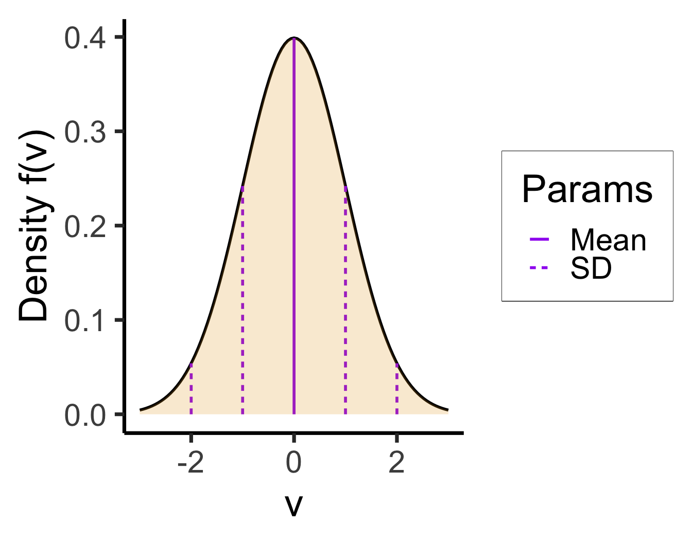
“RV \(X\) is normally distributed with mean \({\color{purple}\mu}\) and standard deviation \({\color{purple}\sigma}\)”
- Translates to \(X \sim \mathcal{N}(\color{purple}{\mu},\color{purple}{\sigma})\)¹
- \(\color{purple}{\mu}\) and \(\color{purple}{\sigma}\) are parameters²: the “knobs” or “sliders” which change the location/shape of the distribution

The parameters in this case give natural summaries of the data:
- \({\color{\purple}\mu}\) = center (mean), \({\color{purple}\sigma}\) = [square root of] variance around center
Mean can usually be interpreted intuitively; for standard deviation, can use the 68-95-99.7 rule, which will make more sense relative to some real-world data…

Real Data and the 68-95-99.7 Rule

Code

library(readr)
height_df <- read_csv("https://gist.githubusercontent.com/jpowerj/9a23807fb71a5f6b6c2f37c09eb92ab3/raw/89fc6b8f0c57e41ebf4ce5cdf2b3cad6b2dd798c/sports_heights.csv")
mean_height <- mean(height_df$height_cm)
sd_height <- sd(height_df$height_cm)
height_density <- function(x) dnorm(x, mean_height, sd_height)
m2_sd <- mean_height - 2 * sd_height
m1_sd <- mean_height - 1 * sd_height
p1_sd <- mean_height + 1 * sd_height
p2_sd <- mean_height + 2 * sd_height
vlines_data <- tibble::tribble(
  ~x, ~xend, ~y, ~yend, ~Params,
  mean_height, mean_height, 0, height_density(mean_height), "Mean",
  m2_sd, m2_sd, 0, height_density(m2_sd), "SD",
  m1_sd, m1_sd, 0, height_density(m1_sd), "SD",
  p1_sd, p1_sd, 0, height_density(p1_sd), "SD",
  p2_sd, p2_sd, 0, height_density(p2_sd), "SD"
)
ggplot(height_df, aes(x = height_cm)) +
    geom_histogram(aes(y = after_stat(density)), binwidth = 5.0) +
    #stat_function(fun = height_density, linewidth = g_linewidth) +
    geom_area(stat = "function", fun = height_density, color="black", linewidth = g_linewidth, fill = cbPalette[1], alpha=0.2) +
    geom_segment(data=vlines_data, aes(x=x, xend=xend, y=y, yend=yend, linetype = Params), linewidth = g_linewidth, color=cbPalette[2]) +
    labs(
      title=paste0("Distribution of heights (cm), N=",nrow(height_df)," athletes\nMean=",round(mean_height,2),", SD=",round(sd_height,2)),
      x="Height (cm)",
      y="Probability Density"
    ) +
    dsan_theme("full")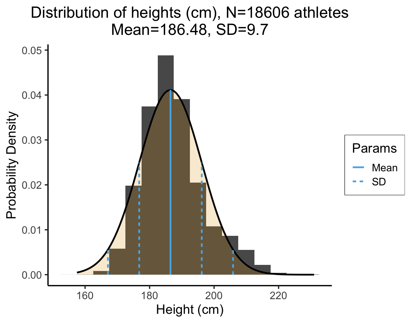

Figure 1: Heights (cm) for 18K professional athletes

Figure 2: 68-95-99.7 Rule visualized (Wiki Commons)

The point estimate \({\color{purple}\mu} = 186.48\) is straightforward: the average height of the athletes is 186.48cm. Using the 68-95-99.7 Rule to interpret the SD, \({\color{purple}\sigma} = 9.7\), we get:

About 68% of the heights fall between

[\({\color{purple}\mu} - 1\cdot {\color{purple}\sigma}\)	and	\({\color{purple}\mu} + 1\cdot {\color{purple}\sigma}\)]
[186.48 - 1 · 9.7	and	186.48 + 1 · 9.7]
[176.78	and	196.18]

About 95% of the heights fall between

[\({\color{purple}\mu} - 2 \cdot {\color{purple}\sigma}\)	and	\({\color{purple}\mu} + 2 \cdot {\color{purple}\sigma}\)]
[186.48 - 2 · 9.7	and	186.48 + 2 · 9.7]
[167.08	and	205.88]

Boxplots: Comparing Multiple Distributions

Another Option: Joyplots

Multivariate Distributions: Preview

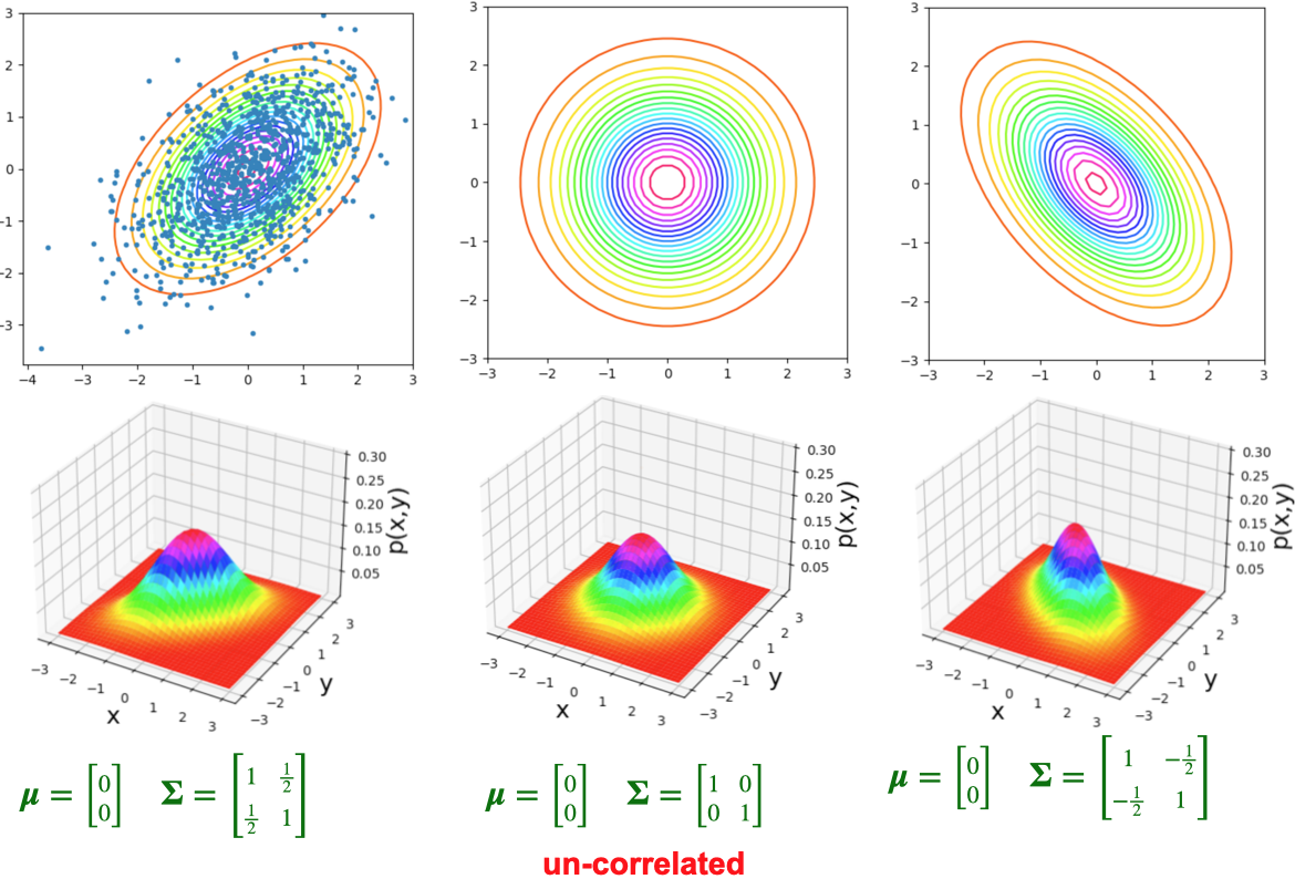
The bivariate normal distribution represents the distribution of two normally-distributed RVs \(\mathbf{X} = [\begin{smallmatrix} X_1 & X_2\end{smallmatrix}]\), which may or may not be correlated:

\[ \mathbf{X} = \begin{bmatrix}X_1 \\ X_2\end{bmatrix}, \; \boldsymbol{\mu} = %\begin{bmatrix}\mu_1 \\ \mu_2\end{bmatrix} \begin{bmatrix}\smash{\overbrace{\mu_1}^{\mathbb{E}[X_1]}} \\ \smash{\underbrace{\mu_2}_{\mathbb{E}[X_2]}}\end{bmatrix} , \; \mathbf{\Sigma} = \begin{bmatrix}\smash{\overbrace{\sigma_1^2}^{\text{Var}[X_1]}} & \smash{\overbrace{\rho\sigma_1\sigma_2}^{\text{Cov}[X_1,X_2]}} \\ \smash{\underbrace{\rho\sigma_2\sigma_1}_{\text{Cov}[X_2,X_1]}} & \smash{\underbrace{\sigma_2^2}_{\text{Var}[X_2]}}\end{bmatrix} % \begin{bmatrix}\sigma_1^2 & \rho\sigma_1\sigma_2 \\ \rho\sigma_2\sigma_1 & \sigma_2^2 \end{bmatrix} % = \begin{bmatrix}\text{Var}[X_1] & \text{Cov}[X_1,X_2] \\ \text{Cov}[X_2,X_1] & \text{Var}[X_2] \end{bmatrix} \]

By squishing all this information intro matrices, we can specify the parameters of multivariate-normally-distributed vectors of RVs similarly to how we specify single-dimensional normally-distributed RVs:

\[ \begin{align*} \overbrace{X}^{\mathclap{\text{scalar}}} &\sim \mathcal{N}\phantom{_k}(\overbrace{\mu}^{\text{scalar}}, \overbrace{\sigma}^{\text{scalar}}) \tag{Univariate} \\ \underbrace{\mathbf{X}}_{\text{vector}} &\sim \boldsymbol{\mathcal{N}}_k(\smash{\underbrace{\boldsymbol{\mu}}_{\text{vector}}}, \underbrace{\mathbf{\Sigma}}_{\text{matrix}}) \tag{Multivariate} \end{align*} \]

Note: In the future I’ll use the notation \(\mathbf{X}_{[a \times b]}\) to denote the dimensions of the vectors/matrices, like \(\mathbf{X}_{[k \times 1]} \sim \boldsymbol{\mathcal{N}}_k(\boldsymbol{\mu}_{[k \times 1]}, \mathbf{\Sigma}_{[k \times k]})\)

Visualizing 3D Distributions: Projection

Most of our intuitions about plots come from 2D \(\Rightarrow\) super helpful exercise to take a 3D plot like this and imagine “projecting” it onto different 2D surfaces:

(Adapted via LaTeX from StackExchange discussion)

Visualizing 3D Distributions: Contours

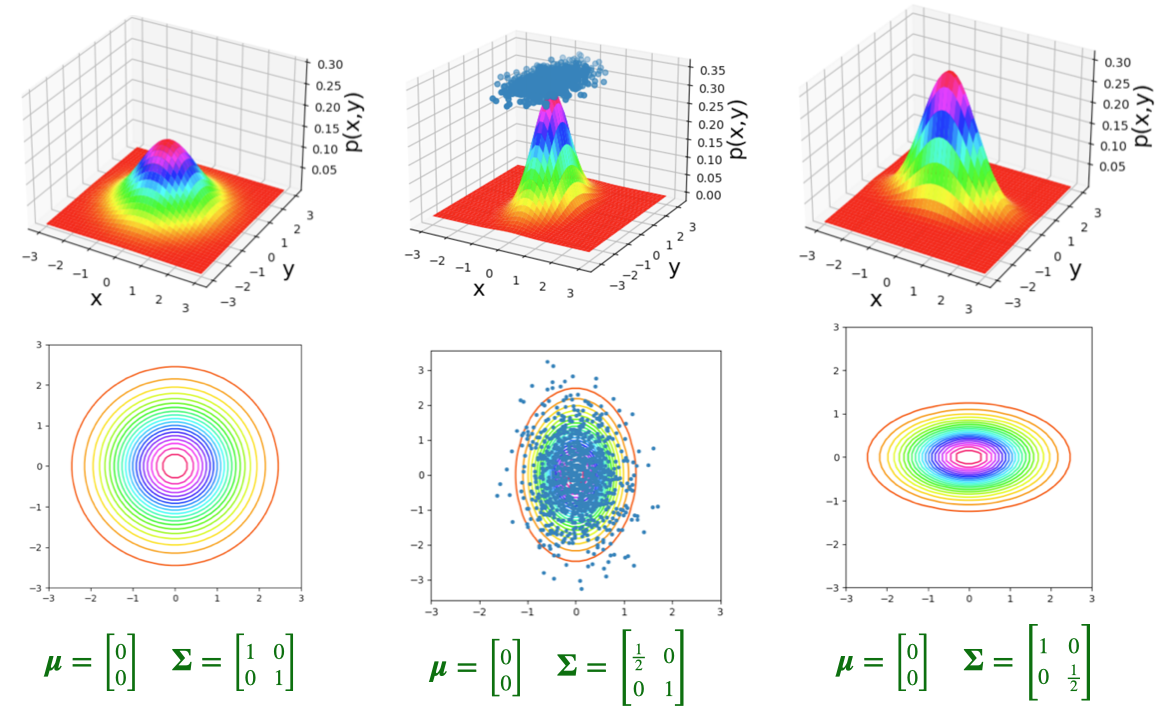
Visualizing 3D Distributions: Contours

“Rules” of Probability

Summarizing What We Know So Far

Logic \(\rightarrow\) Set Theory \(\rightarrow\) Probability Theory
Entirety of probability theory can be derived from two axioms:

The Entirety of Probability Theory Follows From…

Axiom 1 (Unitarity): \(\Pr(\Omega) = 1\) (The probability that something happens is 1)

Axiom 2 (\(\sigma\)-additivity): For mutually-exclusive events \(E_1, E_2, \ldots\),

\[ \underbrace{\Pr\left(\bigcup_{i=1}^{\infty}E_i\right)}_{\Pr(E_1\text{ occurs }\vee E_2\text{ occurs } \vee \cdots)} = \underbrace{\sum_{i=1}^{\infty}\Pr(E_i)}_{\Pr(E_1\text{ occurs}) + \Pr(E_2\text{ occurs}) + \cdots} \]

But what does “mutually exclusive” mean…?

Venn Diagrams: Sets

\[ \begin{align*} &A = \{1, 2, 3\}, \; B = \{4, 5, 6\} \\ &\implies A \cap B = \varnothing \end{align*} \]

\[ \begin{align*} &A = \{1, 2, 3, 4\}, \; B = \{3, 4, 5, 6\} \\ &\implies A \cap B = \{3, 4\} \end{align*} \]

Venn Diagrams: Events (Dice)

\[ \begin{align*} A &= \{\text{Roll is even}\} = \{2, 4, 6\} \\ B &= \{\text{Roll is odd}\} = \{1, 3, 5\} \\ C &= \{\text{Roll is in Fibonnaci sequence}\} = \{1, 2, 3, 5\} \end{align*} \]

Set 1	Set 2	Intersection	Mutually Exclusive?	Can Happen Simultaneously?
\(A\)	\(B\)	\(A \cap B = \varnothing\)	Yes	No
\(A\)	\(C\)	\(A \cap C = \{2\}\)	No	Yes
\(B\)	\(C\)	\(B \cap C = \{1, 3, 5\}\)	No	Yes

“Rules” of Probability

(Remember: not “rules” but “facts resulting from the logic \(\leftrightarrow\) probability connection”)

“Rules” of Probability

For logical predicates \(p, q \in \{T, F\}\), events \(P, Q\) defined so \(P\) = event that \(p\) becomes true, \(Q\) = event that \(q\) becomes true,

Logical AND = Probabilistic Multiplication

\[ \Pr(p \wedge q) = \Pr(P \cap Q) = \Pr(P) \cdot \Pr(Q) \]

Logical OR = Probabilistic Addition

\[ \Pr(p \vee q) = \Pr(P \cup Q) = \Pr(P) + \Pr(Q) - \underbrace{\Pr(P \cap Q)}_{\text{(see rule 1)}} \]

Logical NOT = Probabilistic Complement

\[ \Pr(\neg p) = \Pr(P^c) = 1 - \Pr(P) \]

What is Conditional Probability?

Conditional Probability

Usually if someone asks you probabilistic questions, like
- “What is the likelihood that [our team] wins?”
- “Do you think it will rain tomorrow?”
You don’t guess a random number, you consider and incorporate evidence.
Example: \(\Pr(\text{rain})\) on its own, no other info? Tough question… maybe \(0.5\)?
In reality, we would think about
- \(\Pr(\text{rain} \mid \text{month of the year})\)
- \(\Pr(\text{rain} \mid \text{where we live})\)
- \(\Pr(\text{rain} \mid \text{did it rain yesterday?})\)
Psychologically, breaks down into two steps: (1) Think of baseline probability, (2) Update baseline to incorporate relevant evidence (more on this in a bit…)
Also recall: all probability is conditional probability, even if just conditioned on “something happened” (\(\Omega\), the thing defined so \(\Pr(\Omega) = 1\))

Naïve Definition 2.0

[Slightly Less] Naïve Definition of Probability

\[ \Pr(A \mid B) = \frac{\text{\# of Desired Outcomes in world where }B\text{ happened}}{\text{\# Total outcomes in world where }B\text{ happened}} = \frac{|B \cap A|}{|B|} \]

World Name	Weather in World	Likelihood of Rain Today
\(R\)	Rained for the past 5 days	\(\Pr(\text{rain} \mid R) > 0.5\)
\(M\)	Mix of rain and non-rain over past 5 days	\(\Pr(\text{rain} \mid M) \approx 0.5\)
\(S\)	Sunny for the past 5 days	\(\Pr(\text{rain} \mid S) < 0.5\)

Law of Total Probability

Suppose the events \(B_1, \ldots, B_k\) form a partition of the space \(\Omega\) and \(\Pr(B_j) > 0 \forall j\).
Then, for every event \(A\) in \(\Omega\),

\[ \Pr(A) = \sum_{i=1}^k \Pr(B_j)\Pr(A \mid B_j) \]
Probability of an event is the sum of its conditional probabilities across all conditions.
In other words: \(A\) is some event, \(B_1, \ldots, B_n\) are mutually exclusive events filling entire sample-space, then

\[ \Pr(A) = \Pr(A \mid B_1)\Pr(B_1) + \Pr(A \mid B_2)\Pr(B_2) + \cdots + \Pr(A \mid B_n)\Pr(B_n) \]

i.e. Compute the probability by summing over all possible cases.

Draw pic on board!

Example

Probability of completing job on time with and without rain: 0.42 and 0.9.
Probability of rain is 0.45. What is probability job will be completed on time?
\(A\) = job will be completed on time, \(B\) = rain

\[ \Pr(B) = 0.45 \implies \Pr(B^c) = 1 - \Pr(B) = 0.55. \]

Note: Events \(B\) and \(B^c\) are exclusive and form partitions of the sample space \(S\)
We know \(\Pr(A \mid B) = 0.24\), \(\Pr(A \mid B^c) = 0.9\).
By the Law of Total Probability, we have

\[ \begin{align*} \Pr(A) &= \Pr(B)\Pr(A \mid B) + \Pr(B^c)\Pr(A \mid B^c) \\ &= 0.45(0.42) + 0.55(0.9) = 0.189 + 0.495 = 0684. \end{align*} \]

So, the probability that the job will be completed on time is 0.684. (source)

Bayes’ Theorem and its Implications

Deriving Bayes’ Theorem

Literally just a re-writing of the conditional probability definition (don’t be scared)!

For two events \(A\) and \(B\), definition of conditional probability says that

\[ \begin{align*} \Pr(A \mid B) &= \frac{\Pr(A \cap B)}{\Pr(B)} \tag{1} \\ \Pr(B \mid A) &= \frac{\Pr(B \cap A)}{\Pr(A)} \tag{2} \end{align*} \]

Multiply to get rid of fractions

\[ \begin{align*} \Pr(A \mid B)\Pr(B) &= \Pr(A \cap B) \tag{1*} \\ \Pr(B \mid A)\Pr(A) &= \Pr(B \cap A) \tag{2*} \end{align*} \]

But set intersection is associative (just like multiplication…), \(A \cap B = B \cap A\)! So, we know LHS of \((\text{1*})\) = LHS of \((\text{2*})\):

\[ \Pr(A \mid B)\Pr(B) = \Pr(B \mid A)\Pr(A) \]

Divide both sides by \(\Pr(B)\) to get a new definition of \(\Pr(A \mid B)\), Bayes’ Theorem!

\[ \boxed{\Pr(A \mid B) = \frac{\Pr(B \mid A)\Pr(A)}{\Pr(B)}} \]

Figure 5: Bayes’ Theorem

Why Is This Helpful?

Bayes’ Theorem

For any two events \(A\) and \(B\), \[ \Pr(A \mid B) = \frac{\Pr(B \mid A)\Pr(A)}{\Pr(B)} \]

In words (as exciting as I can make it, for now): Bayes’ Theorem allows us to take information about \(B \mid A\) and use it to infer information about \(A \mid B\)
It isn’t until you work through some examples that this becomes mind-blowing, the most powerful equation we have for inferring unknowns from knowns…
Consider \(A = \{\text{person has disease}\}\), \(B = \{\text{person tests positive for disease}\}\)
1. Is \(A\) observable on its own? No, but…
2. 1. Is \(B\) observable on its own? Yes, and
  2. Can we infer info about \(A\) from knowing \(B\)? Also Yes, thx Bayes!
3. Therefore, we can use \(B\) to infer information about \(A\), i.e., calculate \(\Pr(A \mid B)\)…

Why Is This Helpful for Data Science?

It merges probability theory and hypothesis testing into a single framework:

\[ \Pr(\text{hypothesis} \mid \text{data}) = \frac{\Pr(\text{data} \mid \text{hypothesis})\Pr(\text{hypothesis})}{\Pr(\text{data})} \]

Probability Forwards and Backwards

Two discrete RVs:
- Weather on a given day, \(W \in \{\textsf{Rain},\textsf{Sun}\}\)
- Action that day, \(A \in \{\textsf{Go}, \textsf{Stay}\}\): go to party or stay in and watch movie
Data-generating process: if \(\textsf{Sun}\), rolls a die \(R\) and goes out unless \(R = 6\). If \(\textsf{Rain}\), flips a coin and goes out if \(\textsf{H}\).
Probabilistic Graphical Model (PGM):

So, if we know \(W = \textsf{Sun}\), what is \(P(A = \textsf{Go})\)? \[ \begin{align*} P(A = \textsf{Go} \mid W) &= 1 - P(R = 6) \\ &= 1 - \frac{1}{6} = \frac{5}{6} \end{align*} \]
Conditional probability lets us go forwards (left to right):

But what if we want to perform inference going backwards?

If we see Ana at the party, we know \(A = \textsf{Go}\)
What does this tell us about the weather?
Intuitively, we should increase our degree of belief that \(W = \textsf{Sun}\). But, by how much?
We don’t know \(P(W \mid A)\), only \(P(A \mid W)\)…

\[ P(W = \textsf{Sun} \mid A = \textsf{Go}) = \frac{\overbrace{P(A = \textsf{Go} \mid W = \textsf{Sun})}^{5/6~ ✅}\overbrace{P(W = \textsf{Sun})}^{❓}}{\underbrace{P(A = \textsf{Go})}_{❓}} \]

We’ve seen \(P(W = \textsf{Sun})\) before, it’s our prior: the probability without having any additional relevant knowledge. So, let’s say 50/50. \(P(W = \textsf{Sun}) = \frac{1}{2}\)
If we lived in Seattle, we could pick \(P(W = \textsf{Sun}) = \frac{1}{4}\)

\[ P(W = \textsf{Sun} \mid A = \textsf{Go}) = \frac{\overbrace{P(A = \textsf{Go} \mid W = \textsf{Sunny})}^{5/6~ ✅}\overbrace{P(W = \textsf{Sun})}^{1/2~ ✅}}{\underbrace{P(A = \textsf{Go})}_{❓}} \]

\(P(A = \textsf{Go})\) is trickier: the probability that Ana goes out regardless of what the weather is. But there are only two possible weather outcomes! So we just compute

\[ \begin{align*} &P(A = \textsf{Go}) = \sum_{\omega \in S(W)}P(A = \textsf{Go}, \omega) = \sum_{\omega \in S(W)}P(A = \textsf{Go} \mid \omega)P(\omega) \\ &= P(A = \textsf{Go} \mid W = \textsf{Rain})P(W = \textsf{Rain}) + P(A = \textsf{Go} \mid W = \textsf{Sun})P(W = \textsf{Sun}) \\ &= \left( \frac{1}{2} \right)\left( \frac{1}{2} \right) + \left( \frac{5}{6} \right)\left( \frac{1}{2} \right) = \frac{1}{4} + \frac{5}{12} = \frac{2}{3} \end{align*} \]

Putting it All Together

\[ \begin{align*} P(W = \textsf{Sun} \mid A = \textsf{Go}) &= \frac{\overbrace{P(A = \textsf{Go} \mid W = \textsf{Sunny})}^{3/4~ ✅}\overbrace{P(W = \textsf{Sun})}^{1/2~ ✅}}{\underbrace{P(A = \textsf{Go})}_{1/2~ ✅}} \\ &= \frac{\left(\frac{3}{4}\right)\left(\frac{1}{2}\right)}{\frac{1}{2}} = \frac{\frac{3}{8}}{\frac{1}{2}} = \frac{3}{4}. \end{align*} \]

Given that we see Ana at the party, we should update our beliefs, so that \(P(W = \textsf{Sun}) = \frac{3}{4}, P(W = \textsf{Rain}) = \frac{1}{4}\).

A Scarier Example

Bo worries he has a rare disease. He takes a test with 99% accuracy and tests positive. What’s the probability Bo has the disease? (Intuition: 99%? …Let’s do the math!)

\(H \in \{\textsf{sick}, \textsf{healthy}\}, T \in \{\textsf{T}^+, \textsf{T}^-\}\)
The test: 99% accurate. \(\Pr(T = \textsf{T}^+ \mid H = \textsf{sick}) = 0.99\), \(\Pr(T = \textsf{T}^- \mid H = \textsf{healthy}) = 0.99\).
The disease: 1 in 10K. \(\Pr(H = \textsf{sick}) = \frac{1}{10000}\)
What do we want to know? \(\Pr(H = \textsf{sick} \mid T = \textsf{T}^+)\)
How do we get there?

This photo, originally thought to be of Thomas Bayes, turns out to be probably someone else… \(\Pr(\textsf{Bayes})\)?

\(H\) for health, \(T\) for test result

Photo credit: https://thedatascientist.com/wp-content/uploads/2019/04/reverend-thomas-bayes.jpg

\[ \begin{align*} \Pr(H = \textsf{sick} \mid T = \textsf{T}^+) &= \frac{\Pr(T = \textsf{T}^+ \mid H = \textsf{sick})\Pr(H = \textsf{sick})}{\Pr(T = \textsf{T}^+)} \\ &= \frac{(0.99)\left(\frac{1}{10000}\right)}{(0.99)\left( \frac{1}{10000} \right) + (0.01)\left( \frac{9999}{10000} \right)} \end{align*} \]

p_sick <- 1 / 10000
p_healthy <- 1 - p_sick
p_pos_given_sick <- 0.99
p_neg_given_sick <- 1 - p_pos_given_sick
p_neg_given_healthy <- 0.99
p_pos_given_healthy <- 1 - p_neg_given_healthy
numer <- p_pos_given_sick * p_sick
denom1 <- numer
denom2 <- p_pos_given_healthy * p_healthy
final_prob <- numer / (denom1 + denom2)
final_prob

[1] 0.009803922

… Less than 1% 😱

Proof in the Pudding

Let’s generate a dataset of 5,000 people, using \(\Pr(\textsf{Disease}) = \frac{1}{10000}\)

Code

library(tibble)
library(dplyr)
# Disease rarity
p_disease <- 1 / 10000
# 1K people
num_people <- 10000
# Give them ids
ppl_df <- tibble(id=seq(1,num_people))
# Whether they have the disease or not
has_disease <- rbinom(num_people, 1, p_disease)
ppl_df <- ppl_df %>% mutate(has_disease=has_disease)
ppl_df |> head()

id	has_disease
1	0
2	0
3	0
4	0
5	0
6	0

Binary Variable Trick

Since has_disease \(\in \{0, 1\}\), we can use
- sum(has_disease) to obtain the count of people with the disease, or
- mean(has_disease) to obtain the proportion of people who have the disease
To see this (or, if you forget in the future), just make a fake dataset with a binary variable and 3 rows, and think about sums vs. means of that variable:

Code

binary_df <- tibble(
  id=c(1,2,3),
  x=c(0,1,0)
)
binary_df

id	x
1	0
2	1
3	0

Taking the sum tells us: one row where x == 1:

Code

sum(binary_df$x)

[1] 1

Taking the mean tells us: 1/3 of rows have x == 1:

Code

mean(binary_df$x)

[1] 0.3333333

Applying This to the Disease Data

If we want the number of people who have the disease:

Code

# Compute the *number* of people who have the disease
sum(ppl_df$has_disease)

[1] 1

If we want the proportion of people who have the disease:

Code

# Compute the *proportion* of people who have the disease
mean(ppl_df$has_disease)

[1] 1e-04

(And if you dislike scientific notation like I do…)

Code

format(mean(ppl_df$has_disease), scientific = FALSE)

[1] "0.0001"

(Foreshadowing Monte Carlo methods)

Data-Generating Process: Test Results

Code

library(dplyr)
# Data Generating Process
take_test <- function(is_sick) {
  if (is_sick) {
    return(rbinom(1,1,p_pos_given_sick))
  } else {
    return(rbinom(1,1,p_pos_given_healthy))
  }
}
ppl_df['test_result'] <- unlist(lapply(ppl_df$has_disease, take_test))
num_positive <- sum(ppl_df$test_result)
p_positive <- mean(ppl_df$test_result)
writeLines(paste0(num_positive," positive tests / ",num_people," total = ",p_positive))

112 positive tests / 10000 total = 0.0112

#disp(ppl_df %>% head(50), obs_per_page = 3)
ppl_df |> head()

id	has_disease	test_result
1	0	0
2	0	0
3	0	0
4	0	0
5	0	0
6	0	0

Zooming In On Positive Tests

pos_ppl <- ppl_df %>% filter(test_result == 1)
#disp(pos_ppl, obs_per_page = 10)
pos_ppl |> head()

id	has_disease	test_result
94	0	1
165	0	1
234	0	1
238	0	1
245	0	1
305	0	1

Bo doesn’t have it, and neither do 110 of the 111 total people who tested positive!
But, in the real world, we only observe \(T\)

Zooming In On Disease-Havers

What if we look at only those who actually have the disease? Maybe the cost of 111 people panicking is worth it if we correctly catch those who do have it?

Code

#disp(ppl_df[ppl_df$has_disease == 1,])
ppl_df[ppl_df$has_disease == 1,]

id	has_disease	test_result
8902	1	1

Is this always going to be the case?

Num with disease: 0
Proportion with disease: 0
Number of positive tests: 52

id	has_disease	test_result

#disp(simulate_disease(5000, 1/10000))
simulate_disease(5000, 1/10000)

Num with disease: 0
Proportion with disease: 0
Number of positive tests: 46

id	has_disease	test_result

Worst-Case Worlds

for (i in seq(1,1000)) {
  sim_result <- simulate_disease(5000, 1/10000, verbose = FALSE, return_all_detected = FALSE, return_df = FALSE, return_info = TRUE)
  if (!sim_result$all_detected) {
    writeLines(paste0("World #",i," / 1000 (",sim_result$num_people," people):"))
    print(sim_result$df)
    writeLines('\n')
  }
}

World #130 / 1000 (5000 people):
# A tibble: 1 × 3
     id has_disease test_result
  <int>       <int>       <int>
1  3860           1           0


World #332 / 1000 (5000 people):
# A tibble: 1 × 3
     id has_disease test_result
  <int>       <int>       <int>
1  1046           1           0


World #853 / 1000 (5000 people):
# A tibble: 1 × 3
     id has_disease test_result
  <int>       <int>       <int>
1  4955           1           0

format(4 / 5000000, scientific = FALSE)

[1] "0.0000008"

How unlikely is this? Math:

\[ \begin{align*} \Pr(\textsf{T}^- \cap \textsf{Sick}) &= \Pr(\textsf{T}^- \mid \textsf{Sick})\Pr(\textsf{Sick}) \\ &= (0.01)\frac{1}{10000} \\ &= \frac{1}{1000000} \end{align*} \]

Computers:

result_df <- simulate_disease(1000000, 1/10000, verbose = FALSE, return_full_df = TRUE)
false_negatives <- result_df[result_df$has_disease == 1 & result_df$test_result == 0,]
num_false_negatives <- nrow(false_negatives)
writeLines(paste0("False Negatives: ",num_false_negatives,", Total Cases: ", nrow(result_df)))

False Negatives: 0, Total Cases: 1000000

false_negative_rate <- num_false_negatives / nrow(result_df)
false_negative_rate_decimal <- format(false_negative_rate, scientific = FALSE)
writeLines(paste0("False Negative Rate: ", false_negative_rate_decimal))

False Negative Rate: 0

(Perfect match!)

Bayes: Takeaway

Bayesian approach allows new evidence to be weighed against existing evidence, with statistically principled way to derive these weights:

\[ \begin{array}{ccccc} \Pr_{\text{post}}(\mathcal{H}) &\hspace{-6mm}\propto &\hspace{-6mm} \Pr(X \mid \mathcal{H}) &\hspace{-6mm} \times &\hspace{-6mm} \Pr_{\text{pre}}(\mathcal{H}) \\ \text{Posterior} &\hspace{-6mm}\propto &\hspace{-6mm}\text{Evidence} &\hspace{-6mm} \times &\hspace{-6mm} \text{Prior} \end{array} \]

Monte Carlo Methods: Overview

You already saw an example, in our rare disease simulation!
Generally, using computers (rather than math, “by hand”) to estimate probabilistic quantities

Pros:

Most real-world processes have no analytic solution
Step-by-step breakdown of complex processes

Cons:

Can require immense computing power
⚠️ Can generate incorrect answers ⚠️

By step-by-step I mean, a lot of the time you are just walking through, generating the next column using previously-generated columns. Like we did in the example above, generating test_result based on has_disease.

Birthday Problem

30 people gather in a room together. What is the probability that two of them share the same birthday?
Analytic solution is fun, but requires some thought… Monte Carlo it!

Code

gen_bday_room <- function(room_num=NULL) {
  num_people <- 30
  num_days <- 366
  ppl_df <- tibble(id=seq(1,num_people))
birthdays <- sample(1:num_days, num_people,replace = T)
  ppl_df['birthday'] <- birthdays
  if (!is.null(room_num)) {
    ppl_df <- ppl_df %>% mutate(room_num=room_num) %>% relocate(room_num)
  }
  return(ppl_df)
}
ppl_df <- gen_bday_room(1)
#disp(ppl_df %>% head())
ppl_df |> head()

room_num	id	birthday
1	1	223
1	2	349
1	3	158
1	4	315
1	5	360
1	6	307

# Inefficient version (return_num=FALSE) is for: if you want tibbles of *all* shared bdays for each room
get_shared_bdays <- function(df, is_grouped=NULL, return_num=FALSE, return_bool=FALSE) {
  bday_pairs <- tibble()
  for (i in 1:(nrow(df)-1)) {
    i_data <- df[i,]
    i_bday <- i_data$birthday
    for (j in (i+1):nrow(df)) {
      j_data <- df[j,]
      j_bday <- j_data$birthday
      # Check if they're the same
      same_bday <- i_bday == j_bday
      if (same_bday) {
        if (return_bool) {
          return(1)
        }
        pair_data <- tibble(i=i,j=j,bday=i_bday)
        if (!is.null(is_grouped)) {
          i_room <- i_data$room_num
          pair_data['room'] <- i_room
        }
        bday_pairs <- bind_rows(bday_pairs, pair_data)
      }
    }
  }
  if (return_bool) {
    return(0)
  }
  if (return_num) {
    return(nrow(bday_pairs))
  }
  return(bday_pairs)
}
#get_shared_bdays(ppl_df)
get_shared_bdays(ppl_df)

i	j	bday
13	15	13

Let’s try more rooms…

# Get tibbles for each room
library(purrr)
gen_bday_rooms <- function(num_rooms) {
  rooms_df <- tibble()
  for (r in seq(1, num_rooms)) {
      cur_room <- gen_bday_room(r)
      rooms_df <- bind_rows(rooms_df, cur_room)
  }
  return(rooms_df)
}
num_rooms <- 10
rooms_df <- gen_bday_rooms(num_rooms)
rooms_df %>% group_by(room_num) %>% group_map(~ get_shared_bdays(.x, is_grouped=TRUE))

[[1]]
# A tibble: 0 × 0

[[2]]
# A tibble: 1 × 3
      i     j  bday
  <int> <int> <int>
1    17    29   190

[[3]]
# A tibble: 0 × 0

[[4]]
# A tibble: 2 × 3
      i     j  bday
  <int> <int> <int>
1     6    27   148
2    15    22   282

[[5]]
# A tibble: 1 × 3
      i     j  bday
  <int> <int> <int>
1    14    28    94

[[6]]
# A tibble: 2 × 3
      i     j  bday
  <int> <int> <int>
1     6    15   240
2    10    16   248

[[7]]
# A tibble: 2 × 3
      i     j  bday
  <int> <int> <int>
1     9    17    16
2    19    22   220

[[8]]
# A tibble: 3 × 3
      i     j  bday
  <int> <int> <int>
1     6    20   343
2    17    25    83
3    18    30   249

[[9]]
# A tibble: 0 × 0

[[10]]
# A tibble: 3 × 3
      i     j  bday
  <int> <int> <int>
1     3    23   177
2     5    26    53
3    11    14   286

Number of shared birthdays per room:

# Now just get the # shared bdays
shared_per_room <- rooms_df %>%
    group_by(room_num) %>%
    group_map(~ get_shared_bdays(.x, is_grouped = TRUE, return_num=TRUE))
shared_per_room <- unlist(shared_per_room)
shared_per_room

 [1] 0 1 0 2 1 2 2 3 0 3

\(\widehat{\Pr}(\text{shared})\)

sum(shared_per_room > 0) / num_rooms

[1] 0.7

How about A THOUSAND ROOMS?

num_rooms_many <- 100
many_rooms_df <- gen_bday_rooms(num_rooms_many)
anyshared_per_room <- many_rooms_df %>%
    group_by(room_num) %>%
    group_map(~ get_shared_bdays(.x, is_grouped = TRUE, return_bool = TRUE))
anyshared_per_room <- unlist(anyshared_per_room)
anyshared_per_room

  [1] 1 1 0 1 1 0 0 1 1 1 1 1 1 1 1 1 1 1 1 0 0 1 1 0 1 0 1 1 0 1 1 0 1 1 0 0 1
 [38] 1 1 0 0 1 1 1 0 1 1 1 1 1 1 1 1 1 1 1 0 0 0 0 1 0 0 1 0 1 1 1 1 0 1 1 0 1
 [75] 1 0 0 1 0 1 1 1 1 0 1 1 0 1 0 0 0 1 0 0 1 1 1 1 0 1

\(\widehat{\Pr}(\text{shared bday})\)?

# And now the probability estimate
sum(anyshared_per_room > 0) / num_rooms_many

[1] 0.66

The analytic solution: \(\Pr(\text{shared} \mid k\text{ people in room}) = 1 - \frac{366!}{366^{k}(366-k)!}\)
In our case: \(1 - \frac{366!}{366^{30}(366-30)!} = 1 - \frac{366!}{366^{30}336!} = 1 - \frac{\prod_{i=337}^{366}i}{366^{30}}\)
R can juust barely handle these numbers:

(exact_solution <- 1 - (prod(seq(337,366))) / (366^30))

[1] 0.7053034

Wrapping Up

Source: _bday-solutions-plot.ipynb

Final Note: Functions of Random Variables

\(X \sim U[0,1], Y \sim U[0,1]\).
\(P(Y < X^2)\)?
The hard way: solve analytically
The easy way: simulate!

References

Footnotes

Throughout the course, this “calligraphic” font \(\mathcal{N}\), \(\mathcal{D}\), etc., will be used to denote distributions↩︎
Throughout the course, remember, purrple is for purrameters↩︎