Week 2B: Random Variables
DSAN 5100: Probabilistic Modeling and Statistical Computing
Section 01
Tuesday, September 2, 2025
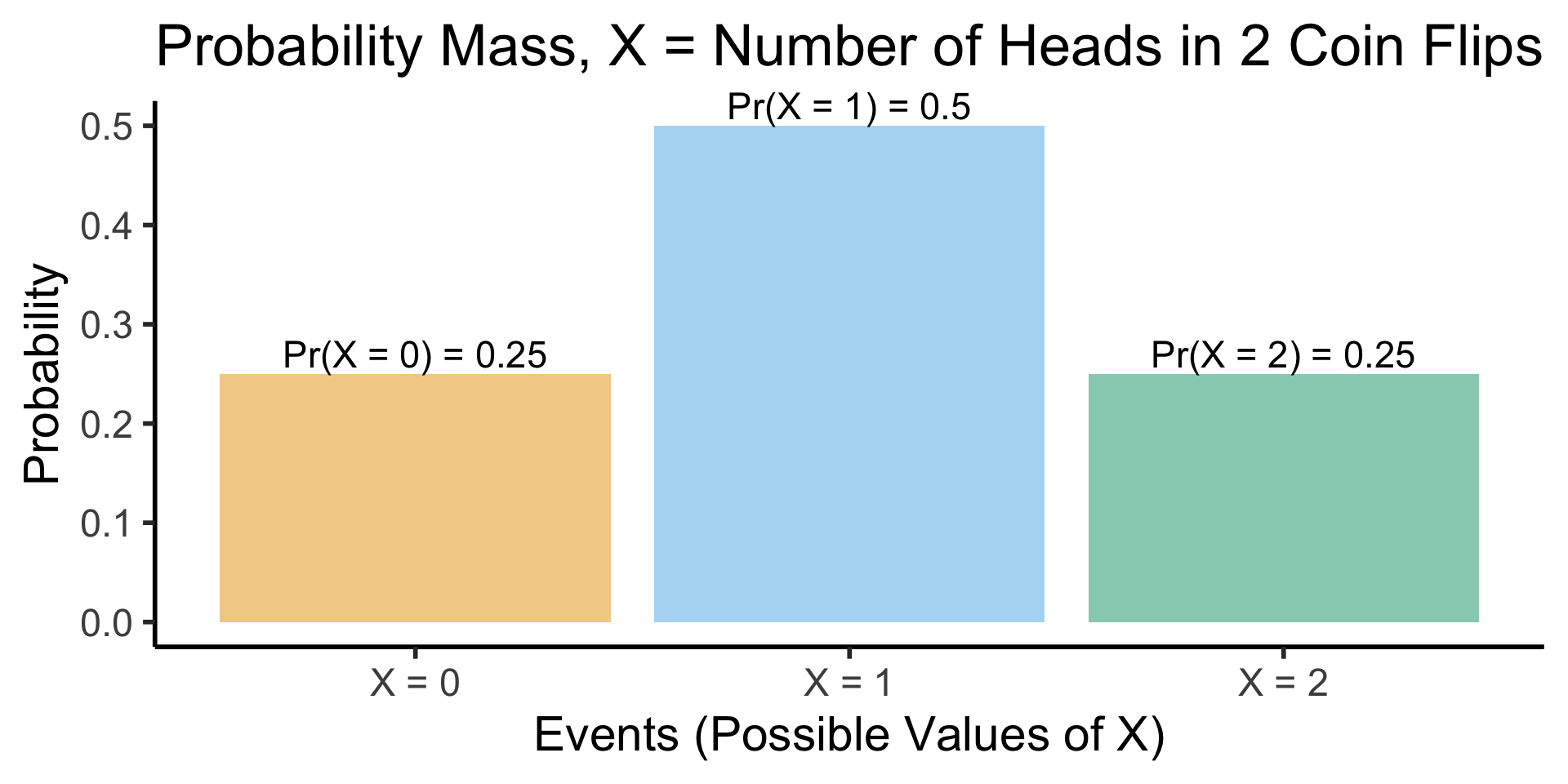
Visualizing Discrete RVs
- Ultimate Probability Pro-Tip: When you hear “discrete distribution”, think of a bar graph: \(x\)-axis = events, bar height = probability of events
- Two coins example: \(X\) = RV representing number of heads obtained in two coin flips
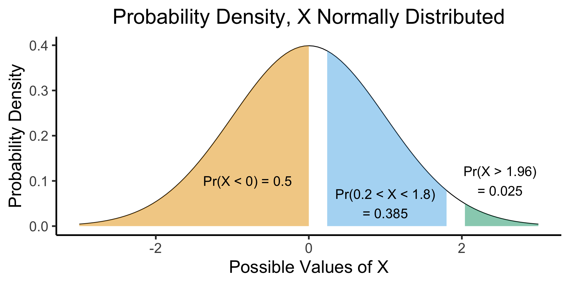
(Preview:) Visualizing Continuous RVs
- This works even for continuous distributions, if you focus on the area under the curve instead of the height:
Example: Game Reviews
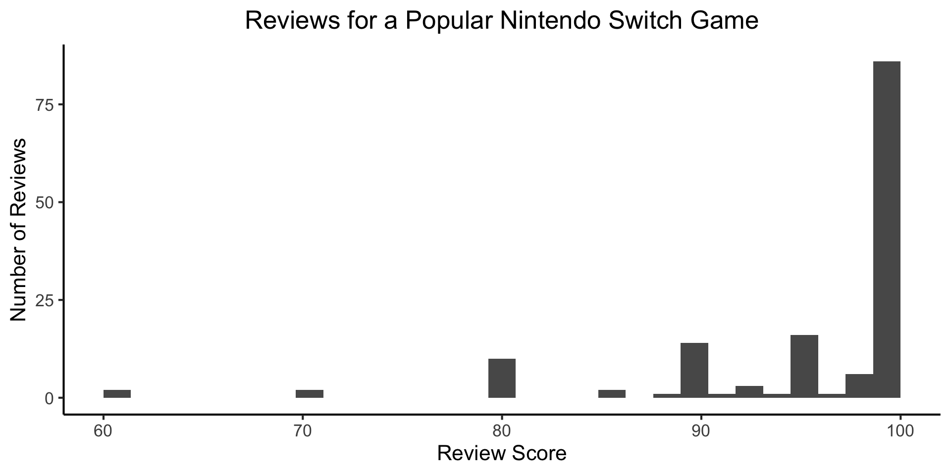
(Data from Metacritic)
Adding a Single Line
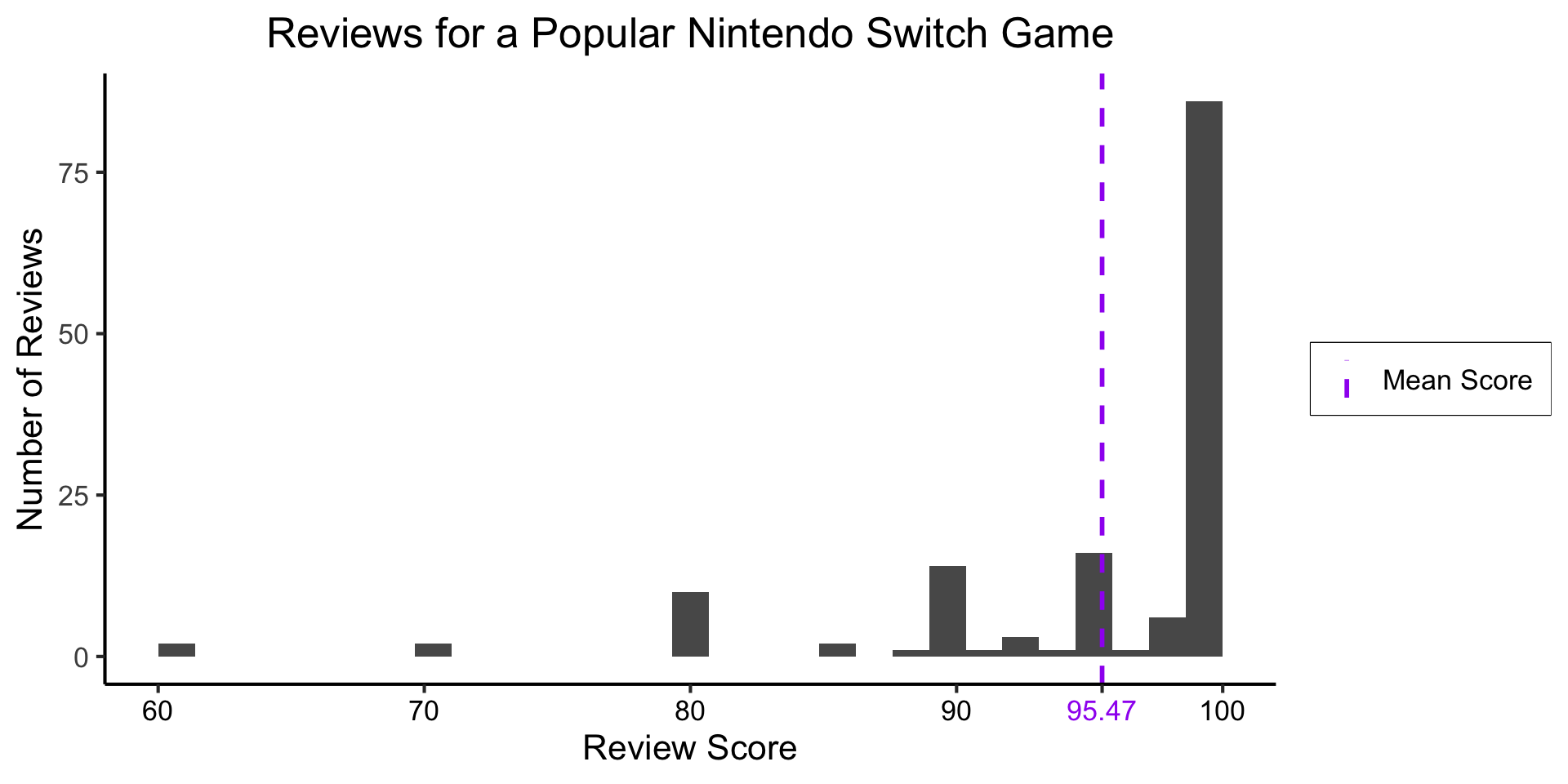
(Data from Metacritic)
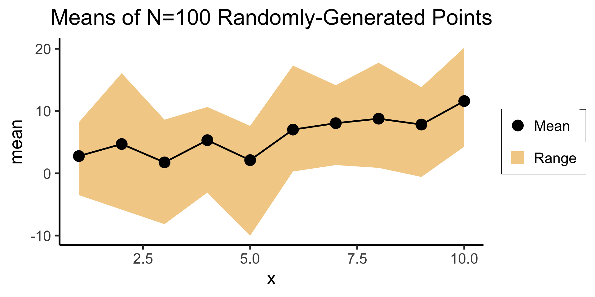
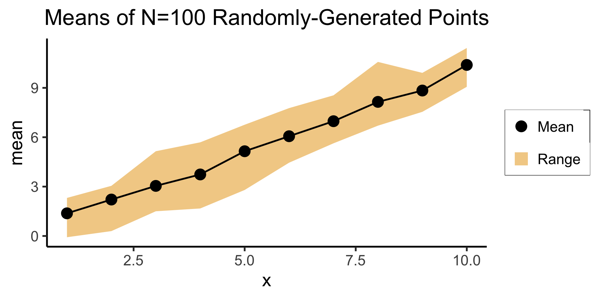
Or a Single Ribbon
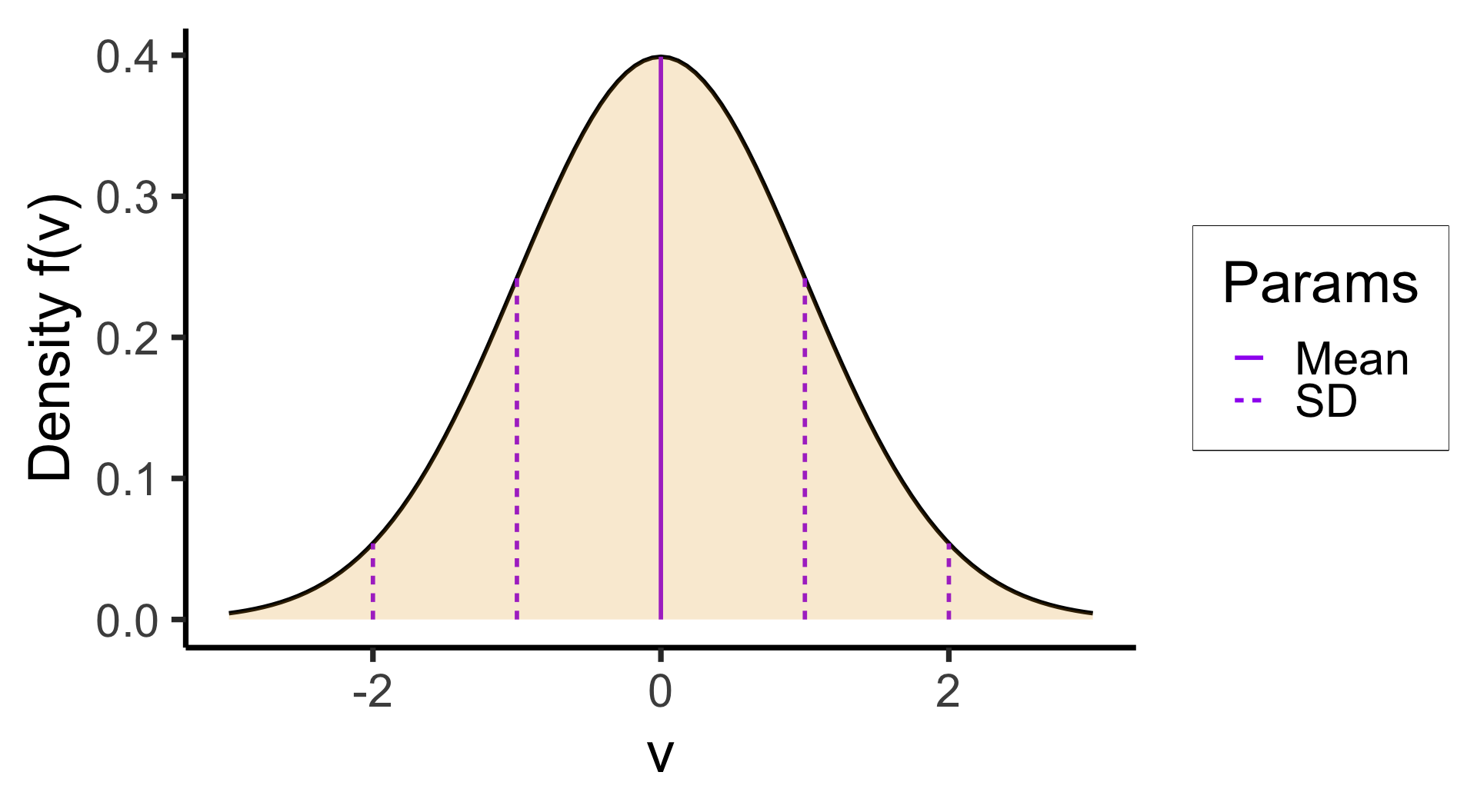
Real Data and the 68-95-99.7 Rule
Code
library(readr)
height_df <- read_csv("https://gist.githubusercontent.com/jpowerj/9a23807fb71a5f6b6c2f37c09eb92ab3/raw/89fc6b8f0c57e41ebf4ce5cdf2b3cad6b2dd798c/sports_heights.csv")
mean_height <- mean(height_df$height_cm)
sd_height <- sd(height_df$height_cm)
height_density <- function(x) dnorm(x, mean_height, sd_height)
m2_sd <- mean_height - 2 * sd_height
m1_sd <- mean_height - 1 * sd_height
p1_sd <- mean_height + 1 * sd_height
p2_sd <- mean_height + 2 * sd_height
vlines_data <- tibble::tribble(
  ~x, ~xend, ~y, ~yend, ~Params,
  mean_height, mean_height, 0, height_density(mean_height), "Mean",
  m2_sd, m2_sd, 0, height_density(m2_sd), "SD",
  m1_sd, m1_sd, 0, height_density(m1_sd), "SD",
  p1_sd, p1_sd, 0, height_density(p1_sd), "SD",
  p2_sd, p2_sd, 0, height_density(p2_sd), "SD"
)
ggplot(height_df, aes(x = height_cm)) +
    geom_histogram(aes(y = after_stat(density)), binwidth = 5.0) +
    #stat_function(fun = height_density, linewidth = g_linewidth) +
    geom_area(stat = "function", fun = height_density, color="black", linewidth = g_linewidth, fill = cbPalette[1], alpha=0.2) +
    geom_segment(data=vlines_data, aes(x=x, xend=xend, y=y, yend=yend, linetype = Params), linewidth = g_linewidth, color=cbPalette[2]) +
    labs(
      title=paste0("Distribution of heights (cm), N=",nrow(height_df)," athletes\nMean=",round(mean_height,2),", SD=",round(sd_height,2)),
      x="Height (cm)",
      y="Probability Density"
    ) +
    dsan_theme("full")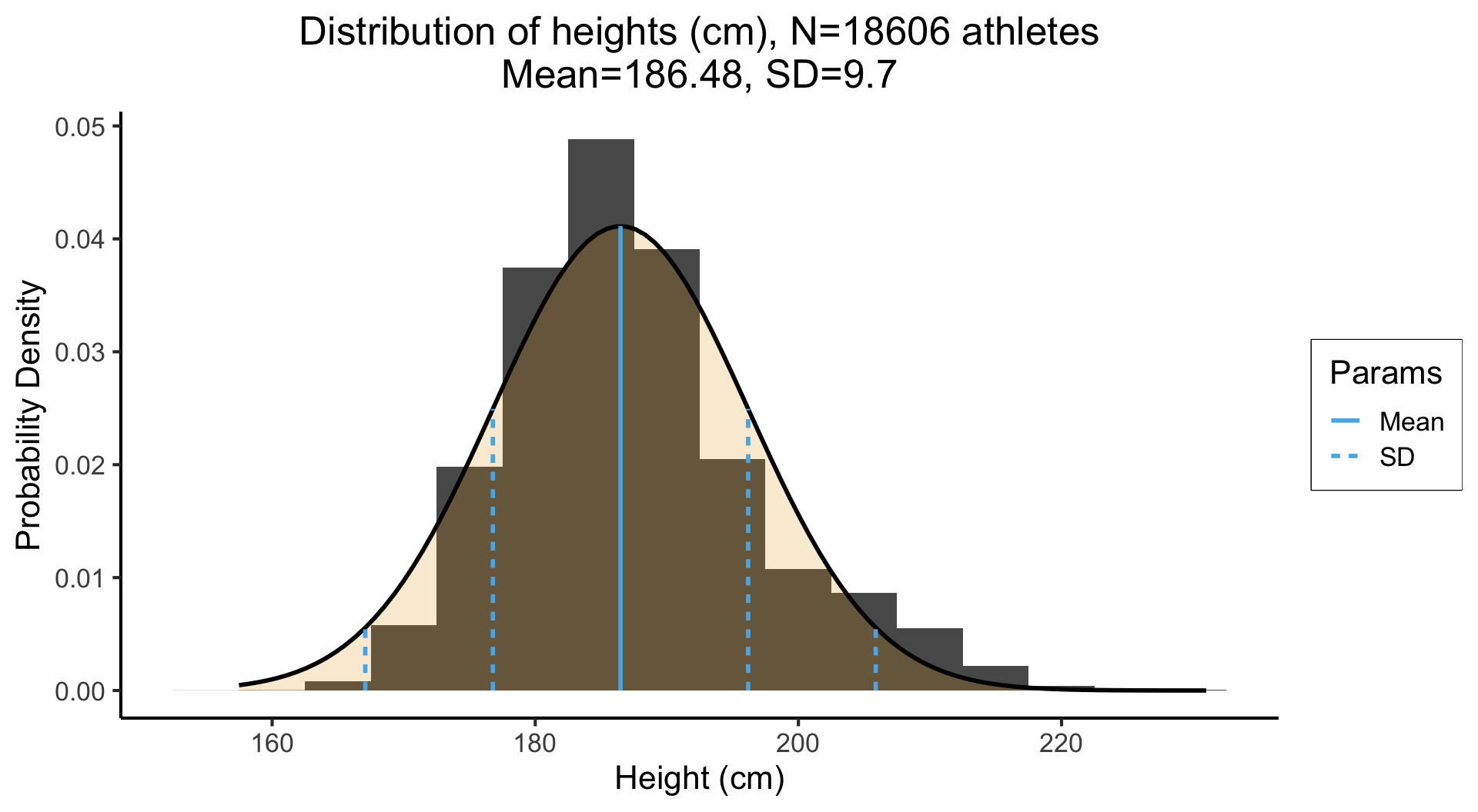

The point estimate \({\color{purple}\mu} = 186.48\) is straightforward: the average height of the athletes is 186.48cm. Using the 68-95-99.7 Rule to interpret the SD, \({\color{purple}\sigma} = 9.7\), we get:
| [\({\color{purple}\mu} - 1\cdot {\color{purple}\sigma}\) | and | \({\color{purple}\mu} + 1\cdot {\color{purple}\sigma}\)] |
| [186.48 - 1 · 9.7 | and | 186.48 + 1 · 9.7] |
| [176.78 | and | 196.18] |
| [\({\color{purple}\mu} - 2 \cdot {\color{purple}\sigma}\) | and | \({\color{purple}\mu} + 2 \cdot {\color{purple}\sigma}\)] |
| [186.48 - 2 · 9.7 | and | 186.48 + 2 · 9.7] |
| [167.08 | and | 205.88] |
Boxplots: Comparing Multiple Distributions


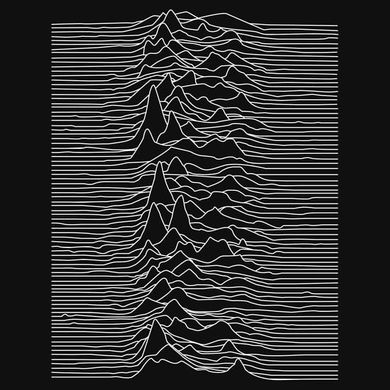
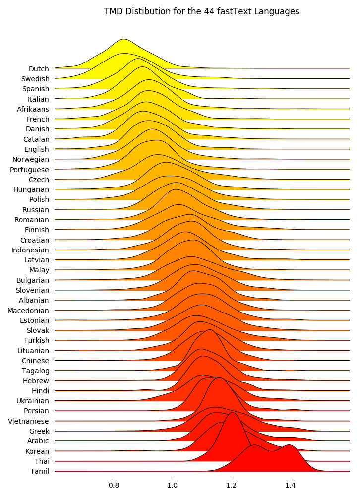
Another Option: Joyplots
Visualizing 3D Distributions: Projection
- Most of our intuitions about plots come from 2D \(\Rightarrow\) super helpful exercise to take a 3D plot like this and imagine “projecting” it onto different 2D surfaces:

(Adapted via LaTeX from StackExchange discussion)
Visualizing 3D Distributions: Contours
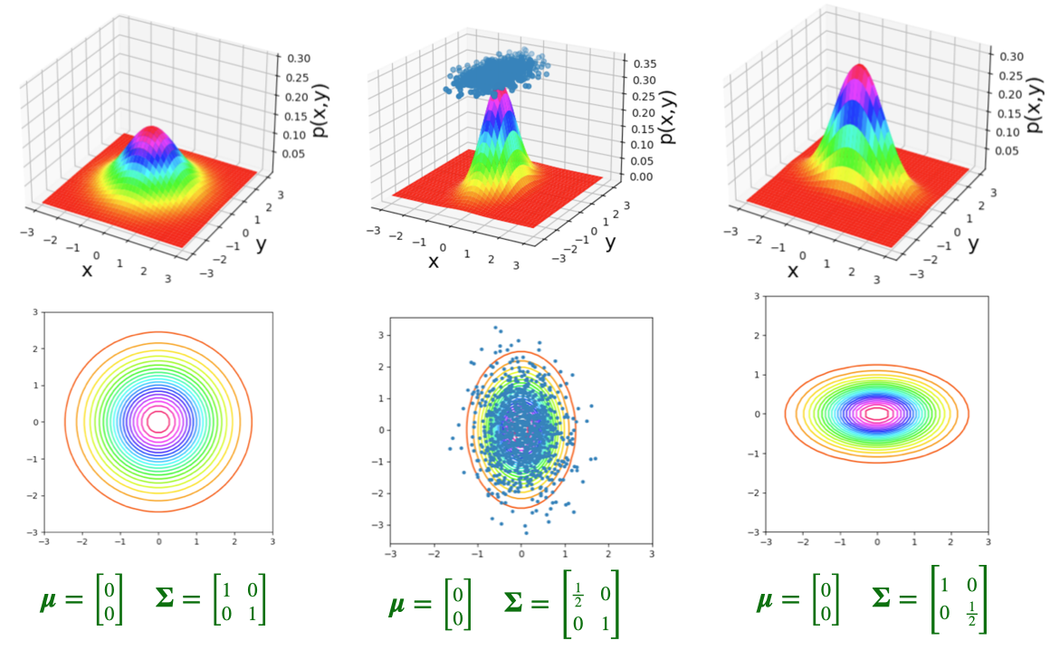
Visualizing 3D Distributions: Contours
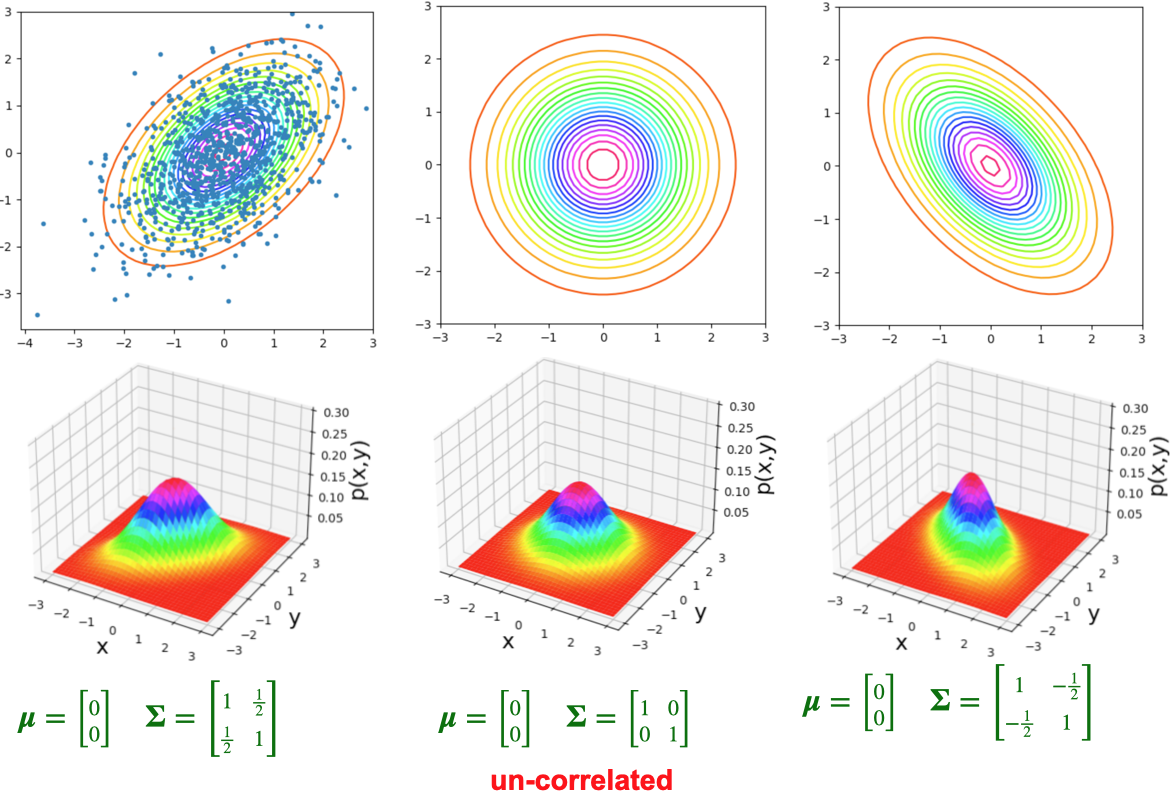
Also from Prof. Hickman’s slides!
Venn Diagrams: Sets
\[ \begin{align*} &A = \{1, 2, 3\}, \; B = \{4, 5, 6\} \\ &\implies A \cap B = \varnothing \end{align*} \]

\[ \begin{align*} &A = \{1, 2, 3, 4\}, \; B = \{3, 4, 5, 6\} \\ &\implies A \cap B = \{3, 4\} \end{align*} \]

Probability Forwards and Backwards
Two discrete RVs:
- Weather on a given day, \(W \in \{\textsf{Rain},\textsf{Sun}\}\)
- Action that day, \(A \in \{\textsf{Go}, \textsf{Stay}\}\): go to party or stay in and watch movie
Data-generating process: if \(\textsf{Sun}\), rolls a die \(R\) and goes out unless \(R = 6\). If \(\textsf{Rain}\), flips a coin and goes out if \(\textsf{H}\).
Probabilistic Graphical Model (PGM):

So, if we know \(W = \textsf{Sun}\), what is \(P(A = \textsf{Go})\)? \[ \begin{align*} P(A = \textsf{Go} \mid W) &= 1 - P(R = 6) \\ &= 1 - \frac{1}{6} = \frac{5}{6} \end{align*} \]
Conditional probability lets us go forwards (left to right):

- If we see Ana at the party, we know \(A = \textsf{Go}\)
- What does this tell us about the weather?
- Intuitively, we should increase our degree of belief that \(W = \textsf{Sun}\). But, by how much?
- We don’t know \(P(W \mid A)\), only \(P(A \mid W)\)…
A Scarier Example
- Bo worries he has a rare disease. He takes a test with 99% accuracy and tests positive. What’s the probability Bo has the disease? (Intuition: 99%? …Let’s do the math!)
- \(H \in \{\textsf{sick}, \textsf{healthy}\}, T \in \{\textsf{T}^+, \textsf{T}^-\}\)
- The test: 99% accurate. \(\Pr(T = \textsf{T}^+ \mid H = \textsf{sick}) = 0.99\), \(\Pr(T = \textsf{T}^- \mid H = \textsf{healthy}) = 0.99\).
- The disease: 1 in 10K. \(\Pr(H = \textsf{sick}) = \frac{1}{10000}\)
- What do we want to know? \(\Pr(H = \textsf{sick} \mid T = \textsf{T}^+)\)
- How do we get there?
Zooming In On Positive Tests
| id | has_disease | test_result |
|---|---|---|
| 108 | 0 | 1 |
| 220 | 1 | 1 |
| 229 | 0 | 1 |
| 236 | 1 | 1 |
| 288 | 0 | 1 |
| 329 | 0 | 1 |
- Bo doesn’t have it, and neither do 110 of the 111 total people who tested positive!
- But, in the real world, we only observe \(T\)

Wrapping Up
