Working with Coordinate Reference Systems (CRS)

PPOL 6805: GIS for Spatial Data Science

The sf library documentation can be a bit vague about how exactly it handles different Coordinate Reference Systems (CRS). The most important pieces of info, though, can be found in the “Values” section within the page for the st_crs() function.

Let’s look at what that part says, in the context of HW2, to see what’s happening “under the hood” when we convert from one CRS to another!

HW2 Question 1.5

Once you complete Question 1.1 to 1.4 on HW1, you will have an object called africa_longlines_sf containing, for each country, the longest LINESTRING out of all of its borders.

Recall how rnaturalearth represents country geometries as MULTIPOLYGONs, since countries like Cape Verde can be made up of multiple POLYGONs! The longest LINESTRING for Cape Verde is therefore just the border around whichever of its islands has the longest coastline, which happens to be Santiago, where its capital city Praia is located.

So, given that definition of the “main” LINESTRING for each country, using mapview to plot your africa_longlines_sf object should produce a map that looks as follows (you can zoom in on Cape Verde, off the coast of Senegal in West Africa, to see the LINESTRING around Santiago):

set.seed(6805)
library(tidyverse) |> suppressPackageStartupMessages()
library(sf) |> suppressPackageStartupMessages()
library(mapview) |> suppressPackageStartupMessages()
if (!(getwd() |> endsWith("working-with-crs"))) {
  setwd("./writeups/working-with-crs")
}
africa_longlines_sf <- readRDS("data/africa_longlines_sf.rds")
africa_longlines_map <- mapview(
  africa_longlines_sf,
  label='geounit'
)
africa_longlines_map

Getting CRS Information

Just looking at that map, there’s not really any easy way to tell what CRS the LINESTRINGs are projected into. The easiest way to get this information is to use the st_crs() function from the sf library! In the following cell we store the result of st_crs() into a variable named africa_longlines_crs, and examine what class this object has:

africa_longlines_crs <- sf::st_crs(africa_longlines_sf)
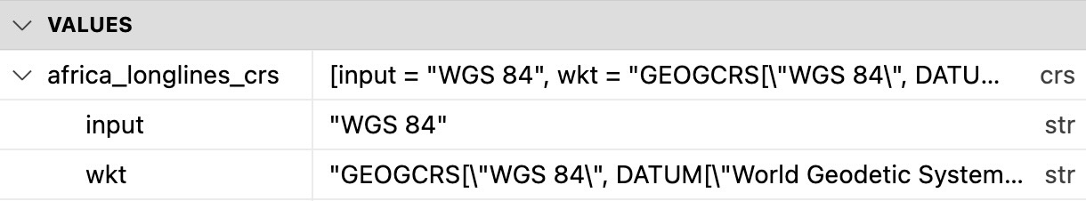
class(africa_longlines_crs)

[1] "crs"

This tells us that st_crs() produces an object of type crs. Which, it turns out, sf does not provide much documentation on, as mentioned above. However, from the page linked above, we can figure out that objects of this crs class will have two pieces of information that we can extract from it: an attribute named input and an attribute named wkt. We can also see this by expanding the africa_longlines_crs entry within the Variables Pane in the bottom-right of Positron’s interface:

We can therefore use print(), or for a way easier-to-read output we can use writeLines() as in the following cell, to display the WKT string for the CRS, that is, all of the information that sf has about the CRS being used:

writeLines(africa_longlines_crs$wkt)

GEOGCRS["WGS 84",
    DATUM["World Geodetic System 1984",
        ELLIPSOID["WGS 84",6378137,298.257223563,
            LENGTHUNIT["metre",1]]],
    PRIMEM["Greenwich",0,
        ANGLEUNIT["degree",0.0174532925199433]],
    CS[ellipsoidal,2],
        AXIS["latitude",north,
            ORDER[1],
            ANGLEUNIT["degree",0.0174532925199433]],
        AXIS["longitude",east,
            ORDER[2],
            ANGLEUNIT["degree",0.0174532925199433]],
    ID["EPSG",4326]]

From this output we can see, at the very bottom, the 4-digit EPSG code for our CRS! If we’d like, we can then use EPSG’s Web API to find even more information about this CRS, by going to https://epsg.io/4326.

The Problem with 4326

Now, if we ask sf to give us a randomly-sampled point along each border as-is, we’ll get an error:

africa_longlines_sf |> sf::st_line_sample(n=1)

Error in sf::st_line_sample(africa_longlines_sf, n = 1): st_line_sample for longitude/latitude not supported; use st_segmentize?

Why is this happening? It’s because (sadly) sf doesn’t support randomly-sampling points from LINESTRINGs which have been projected into the “standard” 4326 CRS.

However, this is an issue specific to the 4326 CRS – if we can re-project each of the geometries in our geom column into a CRS for which sf does support sampling across LINESTRINGs, then we can proceed with our pipeline!

The 1984 → 2020 Updated CRS

It turns out that, as was vaguely mentioned in class, there is another CRS with code 3857 which is slightly more amenable to GIS operations. While the 4326 CRS was created in the 1980s for early GPS systems, the 3857 CRS is regularly updated (most recently in 2020) for ease-of-use with web mapping systems like Google Maps. And, sf can indeed sample points along a LINESTRING if that LINESTRING is projected in CRS 3857.

So, let’s re-project our africa_longlines_sf object into the 3857 CRS, and re-try! We’ll store the result of the st_line_sample() call into a variable named africa_border_points, then we’ll write the last line of our code cell as just africa_border_points so that R outputs the contents of this object as the result of running the cell:

africa_longlines_sf <- africa_longlines_sf |>
  sf::st_transform(3857)
africa_border_points <- africa_longlines_sf |>
  sf::st_line_sample(n=1)
africa_border_points

Geometry set for 54 features 
Geometry type: MULTIPOINT
Dimension:     XY
Bounding box:  xmin: -2645872 ymin: -4074508 xmax: 5619598 ymax: 4276805
Projected CRS: WGS 84 / Pseudo-Mercator
First 5 geometries:

MULTIPOINT ((-189469.2 2627672))

MULTIPOINT ((1437119 -1458796))

MULTIPOINT ((313588.9 1389121))

MULTIPOINT ((2472813 -3048061))

MULTIPOINT ((-471616.7 1484662))

Bam. We can see that, for each of the 54 LINESTRING geometries in our africa_longlines_sf object, it has sampled a single point along this line¹.

We can use mapview() here to generate a quick preview of where each sampled point falls relative to the map of Africa’s borders, to confirm that it has indeed only sampled points along these borders:

africa_points_map <- mapview(
  africa_border_points
)
africa_longlines_map + africa_points_map

Notice how, when you hover your mouse over the points, the popup tooltip just displays a number… that’s because africa_border_points is literally just a bunch of points, indexed by the order in which they were created: Point 1, Point 2, etc. As of now, mapview has no way of knowing that in fact each point is related to a country in africa_longlines_sf! As far as it’s concerned, it is just plotting two unrelated collections of geometries onto the base map of Africa.

So, once you’ve completed Q1.1 through Q1.4, and once you’ve re-projected the LINESTRING geometries within africa_longlines_sf into the 3857 CRS, your remaining task in Q1.5 is to take this africa_border_points object – right now an sfg object² – and add it to africa_longlines_sf as a new column (rather than its own separate object).

Footnotes

1. Note how it creates MULTIPOINT geometries rather than just POINT geometries – this is because sf::st_line_sample() is meant to support sampling any number of points from the line. Thus it always produces a MULTIPOINT geometry, where the number of points within that geometry will be exactly the n parameter we provide to the function. Since we provided n=1, however, the MULTIPOINT only contains a single point, and thus we could safely convert it from MULTIPOINT to POINT without any loss of information (which would also be more memory-efficient, since the sf object would now know that it only has to keep track of a single point for each row!)

2. As briefly mentioned in class, an sfg object is like sf’s version of a “geometric vector”: it is a column that could go into a data.frame or tibble for example, but it also has the special property that it contains WKT-encoded geometries, so that it could also go into an sf object and be used as that sf object’s special geometry column!