ESRI Type: Feature
ESRI Properties: {'OBJECTID': 1, 'area': 41360557.05027756, 'Shape__Area': 413605942350.6803, 'Shape__Length': 4362383.882545892}
Geometry Type: Polygon
First Coordinate: [37.6952778, 39.2168218]PPOL 6805 Week 6 Lab: Interpolating Kurdistan
Labs
Part 1: Overview and Data Loading
Historical Kurdistan Geoms from ESRI
First, check out this amazing ESRI StoryMap, which we’ll cite as Hanson and Hinsdale (2023). If you’re interested, you can read a bunch more about the modern history of the Kurds in McDowall (2021).
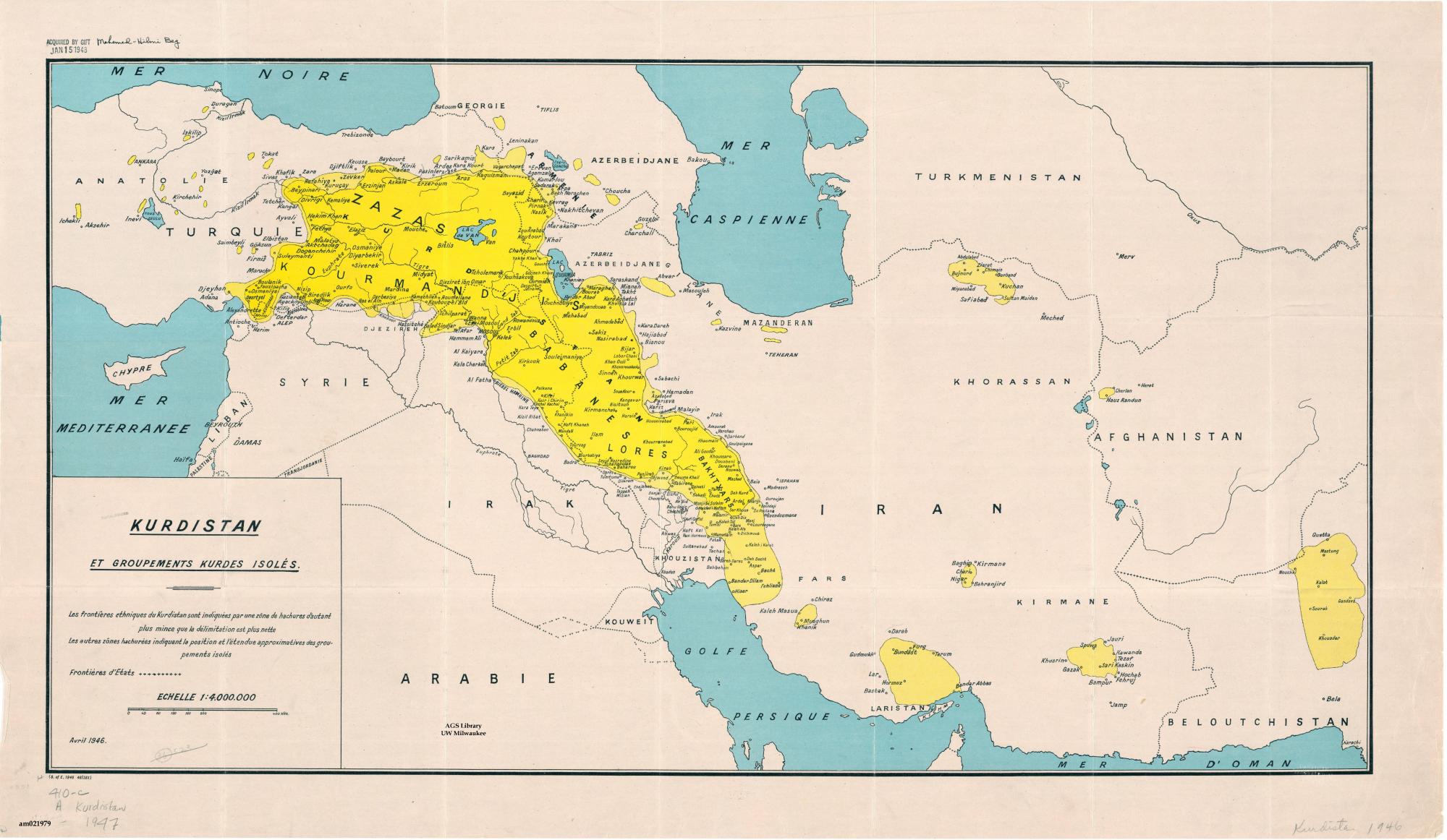
For the sake of this assignment, though, we’ll focus in on the following 1946 map, which Jeff will give the fuller details of (condensing McDowall (2021) into less than 5 minutes, hopefully!) in class:
From ESRI StoryMaps to sf Objects
Digging into the code using Developer Tools reveals the magical API endpoint: https://services.arcgis.com/3xOwF6p0r7IHIjfn/arcgis/rest/services/Kurdistan1947Boundaries
We could wrestle with ESRI’s API, but, there’s an even more fun way, which I learned about via this blog post. Reading that will lead you on to the pyesridump library, which I use within Python to download the layers of that StoryMap as .geojson files.
The details of how pyesridump converts ESRI StoryMap Features into “standard” WKT Geometries can be fun to learn but are a bit outside of the scope of this writeup. But, from the following output you can see that ESRI Features can contain the WKT geometry types we’ve seen (like POINT, LINESTRING, or POLYGON), and in this case the feature we download does indeed correspond to a collection of POLYGONs (here we print just its first coordinate):
The remainder of the lab uses these files, along with rnaturalearth!
Now Modern Border Geoms
library(tidyverse) |> suppressPackageStartupMessages()
library(sf) |> suppressPackageStartupMessages()
library(rnaturalearth) |> suppressPackageStartupMessages()
library(mapview) |> suppressPackageStartupMessages()
country_list <- c(
"Turkey",
"Iran",
"Iraq",
"Syria"
)
countries_sf <- rnaturalearth::ne_countries(
scale=50,
type="countries",
country=country_list
)From among allll the variables in countries_sf, we’re only going to need geounit and (later) pop_est!
countries_sf <- countries_sf |>
  select(geounit, pop_est)
countries_map <- mapview(
countries_sf,
zcol='geounit'
)
countries_mapAnd now the 1946 .geojson file, from the ESRI StoryMap, as discussed above!
print(getwd())[1] "/Users/jpj/gtown-local/ppol6805/writeups/interpolation"if (endsWith(getwd(), "ppol6805")) {
setwd("./writeups/interpolation/")
}
krd_sf <- sf::st_read("data/krd_46.geojson") |>
mutate(label="Kurdistan 1946")Reading layer `krd_46' from data source
`/Users/jpj/gtown-local/ppol6805/writeups/interpolation/data/krd_46.geojson'
using driver `GeoJSON'
Simple feature collection with 1 feature and 4 fields
Geometry type: POLYGON
Dimension: XY
Bounding box: xmin: 36.25249 ymin: 31.58789 xmax: 50.9462 ymax: 40.05815
Geodetic CRS: WGS 84krd_map <- mapview(krd_sf, zcol='label')
krd_mapcountries_map + krd_mapPart 2: Areal-Weighted Interpolation for “Division”
First: Splitting KRD
Intersects as the default predicate… not very helpful here!
default_sf <- countries_sf[krd_sf,]
mapview(default_sf)
But, intersection, via st_intersection(), does give us what we want!
# inter_sf <- st_as_sf(st_union(st_intersection(countries_sf, krd_sf)))
inter_sf <- st_intersection(countries_sf, krd_sf)
Warning: attribute variables are assumed to be spatially constant throughout
all geometriesmapview(inter_sf)New Name Column
inter_sf <- inter_sf |> mutate(
  krd_name = paste0(geounit, " Kurdistan")
)
Now let’s view the four rows of the sf object individually:
mapview(inter_sf[1,], zcol='krd_name')mapview(inter_sf[2,], zcol='krd_name')mapview(inter_sf[3,], zcol='krd_name')mapview(inter_sf[4,], zcol='krd_name')…And All at Once
mapview(inter_sf, zcol='krd_name')Very cool, but, we haven’t taken population into account at all, which was the whole point of this exercise… spatial join / interpolation time!
Spatial Join / Interpolation
Again drawing on McDowall (2021) (this table is on page 4), we can estimate that the overall population across the four modern countries is approximately 32 million:
| Country | % of Country | Count |
|---|---|---|
| Turkey | 18 | 15 million |
| Iran | 10 | 8 million |
| Iraq | 18 | 7.2 million |
| Syria | 9 | 1.8 million |
| Diaspora and Caucasus | - | 2 million |
| Total | - | 34 million |
So, given this estimate, we can now “start over”, this time with the goal of keeping track of the population as we do our operations:
fmt_pop <- function(x) formatC(x,big.mark=",",format='d')
krd_sf <- krd_sf |> mutate(
  pop = 32000000,
  pop_str = fmt_pop(pop)
)
mapview(krd_sf, zcol='pop_str')
Now, if we just use st_intersection()… it doesn’t know that it should pay attention to pop (even if it did know that, it wouldn’t know exactly how you want to split it up… we’ll get there)
pop_intersected_sf <- st_intersection(countries_sf, krd_sf) |>
  mutate(
    pop_str = fmt_pop(pop),
    map_label = paste0(geounit, ' ', pop_str)
  )
Warning: attribute variables are assumed to be spatially constant throughout
all geometriesmapview(pop_intersected_sf, zcol='pop', label='map_label')So… what do we do? The binary operations we’ve learned so far won’t cut it, sadly.
So, we need to cap off the binary operations portion of the class with the fanciest operation we’ll need: spatial joins, though more specifically we’ll want an interpolation. The function in sf is called st_interpolate_aw().
Let’s add that to our toolkit and get to spatial statistics/data science!
pop_interpolated_sf <- st_interpolate_aw(
  krd_sf['pop'],
  countries_sf,
  extensive=TRUE
)
Warning in st_interpolate_aw.sf(krd_sf["pop"], countries_sf, extensive = TRUE):
st_interpolate_aw assumes attributes are constant or uniform over areas of xpop_interpolated_sf| pop | geometry |
|---|---|
| 13967353 | MULTIPOLYGON (((25.97002 40… |
| 749878 | MULTIPOLYGON (((35.89268 35… |
| 5987342 | MULTIPOLYGON (((42.35898 37… |
| 11295426 | MULTIPOLYGON (((56.18799 26… |
And let’s visualize it!
pop_interpolated_sf <- pop_interpolated_sf |> mutate(
  pop_rounded = round(pop, 0),
  pop_str = fmt_pop(pop_rounded)
)
mapview(pop_interpolated_sf, zcol='pop', label='pop_str')
Cool, this tells us, if we didn’t create a Kurdistan, and just drew the borders of the four states (hypothetically…….), how many Kurds would be in each country (again, assuming uniform distribution across 1947 Kurdistan!)
pop_interpolated_sf| pop | geometry | pop_rounded | pop_str |
|---|---|---|---|
| 13967353 | MULTIPOLYGON (((25.97002 40… | 13967353 | 13,967,353 |
| 749878 | MULTIPOLYGON (((35.89268 35… | 749878 | 749,878 |
| 5987342 | MULTIPOLYGON (((42.35898 37… | 5987342 | 5,987,342 |
| 11295426 | MULTIPOLYGON (((56.18799 26… | 11295426 | 11,295,426 |
pop_interpolated_sf$pop |> sum() |> fmt_pop()[1] "32,000,000"Now Interpolating Over the Intersection
I think of the above as kind of a… “partially-spatially-aware” interpolation. This isn’t a great description, but, what I’m getting at is the fact that:
- It does successfully compute how our population (of 1947 Kurdistan) proportionally distributes across the four national borders, but
- It then represents the output, geometrically (as in, the
geometrycolumn), as just the original four countries, now with an additional non-spatial property: the Kurdish population in that country
So, for what I’ll call a “fully-spatially-aware” interpolation, we’ll combine the two things we figured out above:
- Spatial intersection between 1947 Kurdistan and the four countries (producing Turkish, Iranian, Syrian, and Iraqi Kurdistan), plus
- The areal-weighted interpolation we just did above
And it turns out, all that we really need to change is which sf object we’re spatially interpolating across! Meaning, this is the above code, copied-and-pasted, with countries_sf now replaced by inter_sf:
fully_joined_sf <- st_interpolate_aw(
  krd_sf['pop'],
  inter_sf,
  extensive=TRUE
)
Warning in st_interpolate_aw.sf(krd_sf["pop"], inter_sf, extensive = TRUE):
st_interpolate_aw assumes attributes are constant or uniform over areas of xmapview(fully_joined_sf)Also take note of something here: how did mapview “know” to color the four regions by population (using the viridis scheme, the default in mapview!), when we didn’t specify anything for the zcol argument?
This happens because, st_interpolate_aw() is solely dedicated to computing a single piece of information: the population that results from distributing the first argument (numeric) across the second argument (an sf, with a geometry column)! It’s technically not intended to carry out a full-on join.
So, if you find yourself needing to keep all the other information along with the new areal-weighted population (which will usually be the case), just make sure you add the new areal-weighted population column in fully_joined_sf back into the sf object you passed as the second argument to st_interpolate_aw(), as a new column:
inter_sf <- inter_sf |> mutate(
  interpolated_pop = fully_joined_sf$pop
)
inter_sf| geounit | pop_est | OBJECTID | area | Shape__Area | Shape__Length | label | geometry | krd_name | interpolated_pop | |
|---|---|---|---|---|---|---|---|---|---|---|
| 37 | Turkey | 83429615 | 1 | 41360557 | 413605942351 | 4362384 | Kurdistan 1946 | MULTIPOLYGON (((37.746 39.1… | Turkey Kurdistan | 13967353 |
| 47 | Syria | 17070135 | 1 | 41360557 | 413605942351 | 4362384 | Kurdistan 1946 | MULTIPOLYGON (((41.81781 36… | Syria Kurdistan | 749878 |
| 142 | Iraq | 39309783 | 1 | 41360557 | 413605942351 | 4362384 | Kurdistan 1946 | MULTIPOLYGON (((46.56862 32… | Iraq Kurdistan | 5987342 |
| 143 | Iran | 82913906 | 1 | 41360557 | 413605942351 | 4362384 | Kurdistan 1946 | MULTIPOLYGON (((44.54024 39… | Iran Kurdistan | 11295426 |
And now we can use all the other info, like the name, for the rest of our analysis! For example, when making an interactive map!
inter_sf <- inter_sf |> mutate(
  krd_name = paste0(geounit, ' Kurdistan'),
  pop_str = fmt_pop(interpolated_pop),
  krd_label = paste0(krd_name, ': ', pop_str)
)
mapview(inter_sf, zcol='interpolated_pop', label='krd_label')
Part 3: Areal-Weighted Interpolation as “Aggregation”
Part 3.1: Estimating Kurdistan Population from Country Populations
Here, we pretend we don’t know the population of Kurdistan, and try to estimate it from the four country populations, based on how much of each country POLYGONs overlap with the Kurdistan POLYGON:
countries_sf| geounit | pop_est | geometry | |
|---|---|---|---|
| 37 | Turkey | 83429615 | MULTIPOLYGON (((25.97002 40… |
| 47 | Syria | 17070135 | MULTIPOLYGON (((35.89268 35… |
| 142 | Iraq | 39309783 | MULTIPOLYGON (((42.35898 37… |
| 143 | Iran | 82913906 | MULTIPOLYGON (((56.18799 26… |
Visualized:
countries_sf <- countries_sf |> mutate(
  pop_str = fmt_pop(pop_est),
  pop_label = paste0(geounit, ": ", pop_str)
)
mapview(countries_sf, zcol="pop_est", label="pop_label") + krd_map
krd_pop_est_sf <- st_interpolate_aw(
countries_sf['pop_est'],
krd_sf,
extensive = TRUE
)Warning in st_interpolate_aw.sf(countries_sf["pop_est"], krd_sf, extensive =
TRUE): st_interpolate_aw assumes attributes are constant or uniform over areas
of xkrd_sf <- krd_sf |> mutate(
pop_est = krd_pop_est_sf$pop_est,
pop_str = fmt_pop(pop_est),
geounit = "Kurdistan",
pop_label = paste0("Kurdistan Est: ", pop_str)
)
krd_sf| OBJECTID | area | Shape__Area | Shape__Length | geometry | label | pop | pop_str | pop_est | geounit | pop_label |
|---|---|---|---|---|---|---|---|---|---|---|
| 1 | 41360557 | 413605942351 | 4362384 | POLYGON ((37.69528 39.21682… | Kurdistan 1946 | 3.2e+07 | 34,607,914 | 34607915 | Kurdistan | Kurdistan Est: 34,607,914 |
And, visualized!
mapview(countries_sf, zcol="pop_est", label="pop_label") + mapview(krd_sf, zcol="pop_est", label="pop_label")We can also just combine our estimated Kurdistan data with the country data into one, big sf object with 5 rows, where we just have to keep in mind that we’ve technically changed the unit of observation in each row from “UN-recognized country” to essentially “Geopolitical entity of some sort”
krd_sub_sf <- krd_sf |> select(
  geounit, pop_est, pop_str, pop_label
)
pol_ent_sf <- rbind(countries_sf, krd_sub_sf)
pol_ent_sf| geounit | pop_est | pop_str | pop_label | geometry | |
|---|---|---|---|---|---|
| 37 | Turkey | 83429615 | 83,429,615 | Turkey: 83,429,615 | MULTIPOLYGON (((25.97002 40… |
| 47 | Syria | 17070135 | 17,070,135 | Syria: 17,070,135 | MULTIPOLYGON (((35.89268 35… |
| 142 | Iraq | 39309783 | 39,309,783 | Iraq: 39,309,783 | MULTIPOLYGON (((42.35898 37… |
| 143 | Iran | 82913906 | 82,913,906 | Iran: 82,913,906 | MULTIPOLYGON (((56.18799 26… |
| 1 | Kurdistan | 34607915 | 34,607,914 | Kurdistan Est: 34,607,914 | POLYGON ((37.69528 39.21682… |
And now, with a single mapview call:
mapview(pol_ent_sf, zcol='pop_est', label='pop_label')Part 4: Calibrating Two Grids
There is a “Northern” Kurdish language, Kurmanji, as well as a “Central” Kurdish language called Sorani1 While it’s a bit difficult (though, very possible!) to get POLYGONs for language groups, there are standardized datasets like Glottolog and WALS that we can use to get at least the centroid of where the language is spoken, as a POINT:
kl_df <- tibble::tribble(
  ~name, ~lat, ~lon,
  # "Northern" Kurdish language: Kurmanji
  "Kurmanji Centroid", 37.00, 43.00,
  # "Central" Kurdish language: Sorani
  "Sorani Centroid", 35.65, 45.81
)
# sf for language centroids
kl_cent_sf <- st_as_sf(
  kl_df,
  coords=c('lon','lat'),
  crs=4326
)
(cent_map <- mapview(kl_cent_sf))
So, let’s use Voronoi tessellation to split Kurdistan into two sections, based on whether each point is closer to the Kurmanji or Sorani centroid!
krd_voronoi <- st_voronoi(
  st_union(kl_cent_sf),
  envelope=st_as_sfc(st_bbox(krd_sf))
)
Warning in st_voronoi.sfc(st_union(kl_cent_sf), envelope =
st_as_sfc(st_bbox(krd_sf))): st_voronoi does not correctly triangulate
longitude/latitude datakrd_extracted <- st_collection_extract(krd_voronoi, "POLYGON")
#mapview(krd_extracted)
krd_inter_sf <- st_sf(geometry = krd_extracted) |>
st_intersection(krd_sf)Warning: attribute variables are assumed to be spatially constant throughout
all geometrieskrd_inter_sf$label <- c("Kurmanji Speakers", "Sorani Speakers")
mapview(krd_inter_sf, zcol='label') + cent_map#northern_sf <- krd_voronoi[1,]
#southern_sf <- krd_voronoi[2,]
# mapview(northern_sf) + mapview(southern_sf)
#mapview(st_intersection(st_cast(krd_voronoi),krd_sf))So now our job becomes: can we re-do the above estimate of Kurdistan’s population, but this time derive two separate estimates, where the original estimate is “chopped” into two pieces on the basis of the distribution of area between Kurmanji and Sorani…
The answer is: yes! That’s also the job of st_interpolate_aw() 😎
lang_pop_sf <- st_interpolate_aw(
  countries_sf['pop_est'],
  krd_inter_sf,
  extensive=TRUE
)
Warning in st_interpolate_aw.sf(countries_sf["pop_est"], krd_inter_sf,
extensive = TRUE): st_interpolate_aw assumes attributes are constant or uniform
over areas of xmapview(lang_pop_sf)And, adding back into our krd_inter_sf object so we have all the data “carried over”:
krd_inter_sf <- krd_inter_sf |> mutate(
  pop_est = lang_pop_sf$pop_est,
  pop_str = fmt_pop(pop_est),
  pop_label = paste0(label, ": ", pop_str)
)
mapview(krd_inter_sf, zcol='pop_est', label='pop_label')
Wohoo!
References
Hanson, Gianna, and Lanah Hinsdale. 2023. “Putting Kurdistan on the Map.” ArcGIS StoryMaps.
McDowall, David. 2021. A Modern History of the Kurds. Bloomsbury Academic.