Finding GIS Data

This collection of “core” data sources draws heavily on Chapter 6: “R packages to download open spatial data”, in Moraga (2018), Spatial Statistics for Data Science: Theory and Practice with R

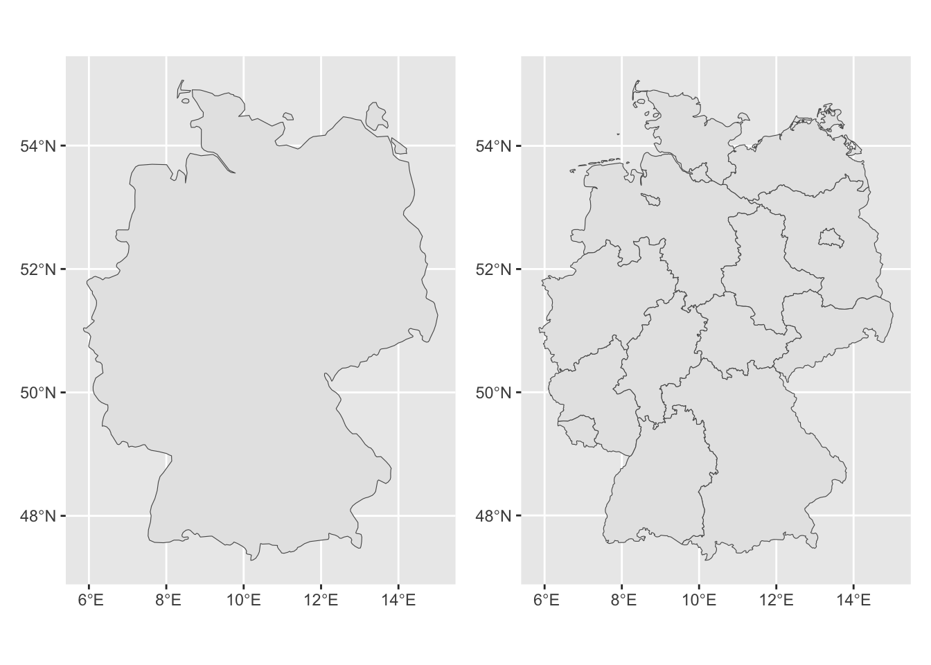
Country Boundaries

Key package: rnaturalearth

library(rnaturalearth)
library(sf) |> suppressPackageStartupMessages()
library(ggplot2)
library(viridis) |> suppressPackageStartupMessages()
library(patchwork)
de_national_map <- ne_countries(type = "countries", country = "Germany", scale = "medium", returnclass = "sf")
de_states_map <- rnaturalearth::ne_states("Germany", returnclass = "sf")
(ggplot(de_national_map) + geom_sf()) + (ggplot(de_states_map) + geom_sf())

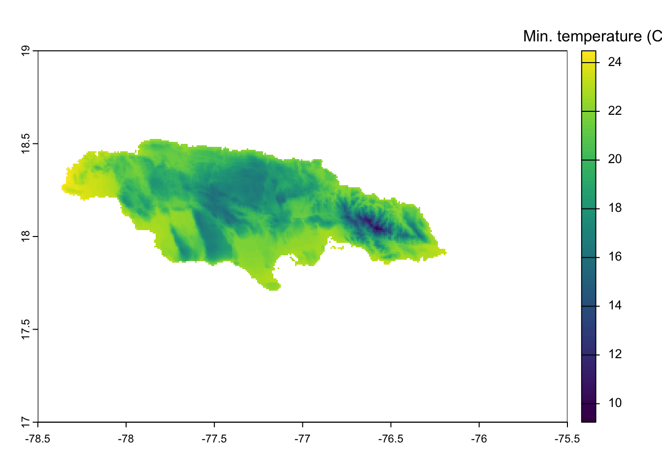
Climate Data

Key package: geodata

library(geodata)

Loading required package: terra

terra 1.8.60

Attaching package: 'terra'

The following object is masked from 'package:patchwork':

    area

jamaica_tmin <- worldclim_country(
  country = "Jamaica",
  var = "tmin",
  path = tempdir()
)
terra::plot(
  mean(jamaica_tmin),
  plg = list(title = "Min. temperature (C)")
)

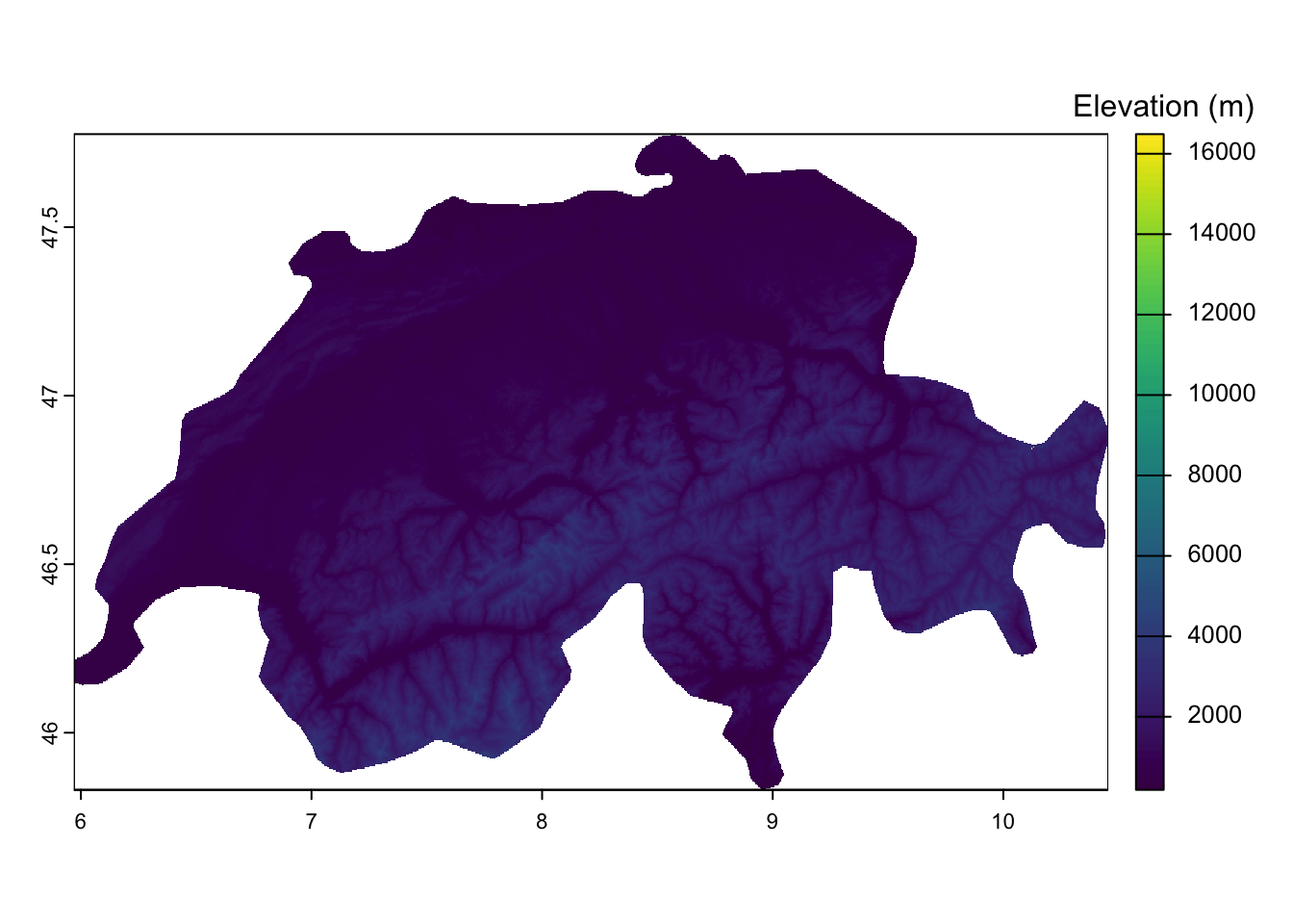
Elevation

Key packages: rnaturalearth + elevatr

library(rnaturalearth)
library(elevatr)

elevatr v0.99.0 NOTE: Version 0.99.0 of 'elevatr' uses 'sf' and 'terra'.  Use 
of the 'sp', 'raster', and underlying 'rgdal' packages by 'elevatr' is being 
deprecated; however, get_elev_raster continues to return a RasterLayer.  This 
will be dropped in future versions, so please plan accordingly.

library(terra)
switz_sf <- ne_countries(
  type = "countries",
  country = "Switzerland",
  scale = "medium",
  returnclass = "sf"
)
# Special weird case with Georgetown's SaxaNet wifi... This if statement just
# tells the R library curl that SaxaNet is indeed a valid wifi connection
if (!curl::has_internet()) {
  assign("has_internet_via_proxy", TRUE, environment(curl::has_internet))
}
switz_raster <- get_elev_raster(
  locations = switz_sf, z = 9, clip = "locations"
)

Mosaicing & Projecting

Clipping DEM to locations

Note: Elevation units are in meters.

terra::plot(
  rast(switz_raster),
  plg = list(title = "Elevation (m)")
)

Street Maps

Key package: osmdata

library(osmdata) |> suppressPackageStartupMessages()
library(leaflet)
placebb <- getbb("Barcelona")
hospitals <- placebb |>
  opq() |>
  add_osm_feature(key = "amenity", value = "hospital") |>
  osmdata_sf()
assign("has_internet_via_proxy", TRUE, environment(curl::has_internet))
motorways <- placebb |>
  opq() |>
  add_osm_feature(
    key = "highway",
    value = "motorway"
  ) |>
  osmdata_sf()
leaflet() |>
  addTiles() |>
  addPolylines(
    data = motorways$osm_lines,
    color = "black"
  ) |>
  addPolygons(
    data = hospitals$osm_polygons,
    label = hospitals$osm_polygons$name
  )

World Bank Dataverse

Key package: wbstats

library(wbstats)
d <- wb_data(
  indicator = "MO.INDEX.HDEV.XQ",
  start_date = 2011, end_date = 2011
)
library(rnaturalearth)
library(mapview)
map <- ne_countries(
  continent = "Africa", returnclass = "sf"
)
map <- dplyr::left_join(
  map, d, by = c("iso_a3" = "iso3c")
)
mapview(map, zcol = "MO.INDEX.HDEV.XQ")

Additional Data Sources (Raindrop.io Bookmarks)