Estimating Legislators’ Ideal Points From Voting Histories

Demos
Published

June 1, 2026

This is an adaptation of an adaptation: my adaptation of BUGS Examples in Stan, which is itself an adaptation of Simon Jackman’s Stan code!

Code
library(pscl) |> suppressPackageStartupMessages()
library(tidyverse) |> suppressPackageStartupMessages()
library(forcats) |> suppressPackageStartupMessages()
library(stringr) |> suppressPackageStartupMessages()
library(rstan) |> suppressPackageStartupMessages()
library(sn) |> suppressPackageStartupMessages()

Recorded votes in legislative settings (roll calls) are often used to recover the underlying preferences of legislators. Political scientists analyze roll call data using the Euclidean spatial voting model: each legislator (\(i = 1, \ldots, n\)) has a preferred policy position (\(x_i\), a point in low-dimensional Euclidean space), and each vote (\(j = 1, \ldots, m\)) amounts to a choice between “Yes” and “No” locations, \(q_j\) and \(Y_j\), respectively. Legislators are assumed to choose on the basis of utility maximization, with one-dimensional utilities.

In these models, the only observed data are votes, and the analyst wants to model those votes as a function of legislator-specific (\(\xi_i\)) and vote-specific (\(\alpha_i\), \(\beta_i\)) parameters.

The vote of legislator \(i\) on roll-call \(j\), \(y_{i,j}\), is a function of the legislator’s ideal point (\(\xi_i\)), the vote’s cutpoint (\(\alpha_j\)), and the vote’s discrimination (\(\beta_j\)):

\[ \begin{aligned}[t] y_{i,j} &\sim \mathsf{Bernoulli}(\pi_i) \\ \pi_i &= \frac{1}{1 + \exp(-\mu_{i,j})} \\ \mu_{i,j} &= \beta_j \xi_i - \alpha_j \end{aligned} \]

Identification

Ideal points (like many latent space models) are unidentified. In particular, there are three types of invariance:

  1. Additive aliasing
  2. Multiplicative aliasing
  3. Rotation (reflection) invariance

Scale invariance:

\[ \begin{aligned}[t] \mu_{i,j} &= \alpha_j + \beta_j \xi_i \\ &= \alpha_j + \left(\frac{\beta_j}{c}\right) \left(\xi_i c \right) \\ &= \alpha_j + \beta^*_j \xi^*_i \end{aligned} \]

Addition invariance:

\[ \begin{aligned}[t] \mu_{i,j} &= \alpha_j + \beta_j \xi_i \\ &= \alpha_j - \beta_j c + \beta_j c + \beta_j \xi_i \\ &= (\alpha_j - \beta_j c) + \beta_j (\xi_i + c) \\ &= \alpha_j^{*} + \beta_j \xi^{*}_i \end{aligned} \]

Rotation invariance:

\[ \begin{aligned}[t] \mu_{i,j} &= \alpha_j + \beta_j \xi_i \\ &= \alpha_j + \beta_j (-1) (-1) \xi_i \\ &= \alpha_j + (-\beta_j) (-\xi_i) \\ &= \alpha_j + \beta_j^{*} \xi^{*}_i \end{aligned} \]

Example:

Code
xi <- c(-1, -0.5, 0.5, 1)
alpha <- c(1, 0, -1)
beta <- c(-0.5, 0, 0.5)
y <- matrix(c(1, 0, 1, 0, 0, 1, 1, 1, 1, 0, 1, 1), 3, 4)
k <- 1

list(
  sum(plogis(y - (alpha + beta %o% xi))),
  sum(plogis(y - (alpha + -beta %o% -xi))),
  sum(plogis(y - ((alpha - beta * k) + beta %o% (xi + k)))),
  sum(plogis(y - ((alpha + (beta / k) %o% (xi * k)))))
)
[[1]]
[1] 7.500395

[[2]]
[1] 7.500395

[[3]]
[1] 7.500395

[[4]]
[1] 7.500395

For each of these: Which types of rotation does it solve?

  1. Fix one element of \(\beta\).
  2. Fix one element of \(\xi\).
  3. Fix one element of \(\alpha\).
  4. Fix two elements of \(\alpha\).
  5. Fix two elements of \(\xi\).
  6. Fix two elements of \(\beta\).

109th Senate

This example models the voting of the 109th U.S. Senate. Votes for the 109th Senate is included in the pscl package:

Code
data("s109", package = "pscl")

The s109 object is not a data frame, so see its documentation for information about its structure.

Code
s109
Description:     109th U.S. Senate 
Source:      ftp://voteview.com/dtaord/sen109kh.ord 
Number of Legislators:   102 
Number of Votes:     645 

Using the following codes to represent roll call votes:
Yea:         1 2 3 
Nay:         4 5 6 
Abstentions:     7 8 9 
Not In Legislature:  0 

Legislator-specific variables:
[1] "state"      "icpsrState" "cd"         "icpsrLegis" "party"     
[6] "partyCode" 
Vote-specific variables:
[1] "date"        "session"     "number"      "bill"        "question"   
[6] "result"      "description" "yeatotal"    "naytotal"   
Detailed information is available via the summary function.

This data includes all roll-call votes, votes in which the responses of the senators are recorded.

For simplicity, the ideal point model uses binary responses, but the s109 data includes multiple codes for responses to roll-calls:

0 not a member
1 Yea
2 Paired Yea
3 Announced Yea
4 Announced Nay
5 Paired Nay
6 Nay
7 Present (some Congresses, also not used some Congresses)
8 Present (some Congresses, also not used some Congresses)
9 Not Voting

In the data processing, we will aggregate the responses into “Yes”, “No”, and missing values.

  • close: Definition of non-lopsided votes in ; votes with between 35% and 65% yeas in which the parties are likely to whip members.
  • lopsided: Definition of lopsided votes used in W-NOMINATE and dropped. Votes with less than 2.5% or greater than 97.5% yeas.
Code
s109_vote_data <- as.data.frame(s109$vote.data) |>
  mutate(
    rollcall = paste(session, number, sep = "-"),
    passed = result %in% c("Confirmed", "Agreed To", "Passed"),
    votestotal = yeatotal + naytotal,
    yea_pct = yeatotal / (yeatotal + naytotal),
    unanimous = yea_pct %in% c(0, 1),
    close = yea_pct < 0.35 | yea_pct > 0.65,
    lopsided = yea_pct < 0.025 | yea_pct > 0.975
  ) |>
  filter(!unanimous) |>
  select(-unanimous) |>
  mutate(.rollcall_id = row_number())
Code
s109_legis_data <- as.data.frame(s109$legis.data) |>
  rownames_to_column("legislator") |>
  mutate(
    .legis_id = row_number(),
    party = fct_recode(
      party,
      "Democratic" = "D",
      "Republican" = "R",
      "Independent" = "Indep"
    )
  )
Code
s109_votes <- s109$votes |>
  as.data.frame() |>
  rownames_to_column("legislator") |>
  gather(rollcall, vote, -legislator) |>
  # recode to Yea (TRUE), Nay (FALSE), or missing
  mutate(
    yea = NA,
    yea = if_else(vote %in% c(1, 2, 3), TRUE, yea),
    yea = if_else(vote %in% c(4, 5, 6), FALSE, yea)
  ) |>
  filter(!is.na(yea)) |>
  inner_join(
    dplyr::select(
      s109_vote_data,
      rollcall,
      .rollcall_id
    ),
    by = "rollcall"
  ) |>
  inner_join(
    dplyr::select(
      s109_legis_data,
      legislator,
      party,
      .legis_id
    ),
    by = "legislator"
  )
s109_votes |> write_csv("s109_votes.csv")
Code
partyline <- s109_votes |>
  group_by(.rollcall_id, party) |>
  summarise(yea = mean(yea)) |>
  spread(party, yea) |>
  ungroup() |>
  mutate(
    partyline = NA_character_,
    partyline = if_else(
      Republican < 0.1 & Democratic > 0.9,
      "Democratic",
      partyline
    ),
    partyline = if_else(
      Republican > 0.9 & Democratic < 0.1,
      "Republican",
      partyline
    )
  ) |>
  rename(
    pct_yea_D = Democratic,
    pct_yea_R = Republican
  ) |>
  select(-Independent)
`summarise()` has regrouped the output.
ℹ Summaries were computed grouped by .rollcall_id and party.
ℹ Output is grouped by .rollcall_id.
ℹ Use `summarise(.groups = "drop_last")` to silence this message.
ℹ Use `summarise(.by = c(.rollcall_id, party))` for per-operation grouping
  (`?dplyr::dplyr_by`) instead.
Code
s109_vote_data <- left_join(
  s109_vote_data,
  partyline,
  by = ".rollcall_id"
)

s109_vote_data |> write_csv("s109_vote_data.csv")

Identification by Fixing Legislator’s Ideal Points

Identification of latent state models can be challenging. The first method for identifying ideal point models is to fix the values of two legislators. These can be arbitrary, but if they are chosen along the ideological dimension of interest it can help the substantive interpretation.

Since we know a priori, or expect, that the primary ideological dimension is Liberal-Conservative (Poole and Rosenthal 2001), I’ll fix the ideal points of the two party leaders in that congress.

In the 109th Congress, the Republican party was the majority party and Bill Frist (Tennessee) was the majority (Republican) leader, and Harry Reid (Nevada) wad the minority (Democratic) leader:

\[ \begin{aligned}[t] \xi_\text{FRIST (R TN)} & = 1 \\ \xi_\text{REID (D NV)} & = -1 \end{aligned} \]

For all of those give a weakly informative prior to the ideal points, and item difficulty and discrimination parameters,

\[ \begin{aligned}[t] \xi_{i} &\sim \mathsf{Normal}(\zeta, \tau) \\ \zeta &\sim \mathsf{Normal}(0., 10) \\ \tau &\sim \mathsf{HalfCauchy}(0., 5) \\ \alpha_{j} &\sim \mathsf{Normal}(0, 10) \\ \beta_{j} &\sim \mathsf{Normal}(0, 2.5) && j \in 1, \dots, J \end{aligned} \]

Code
# mod_ideal_point_1 <- stan_model("stan/ideal_point_1.stan")
Code
# mod_ideal_point_1
// ideal point model
// identification:
// - xi ~ hierarchical
// - except fixed senators
data {
  // number of individuals
  int N;
  // number of items
  int K;
  // observed votes
  int<lower = 0, upper = N * K> Y_obs;
  int y_idx_leg[Y_obs];
  int y_idx_vote[Y_obs];
  int y[Y_obs];
  // priors
  // on items
  real alpha_loc;
  real<lower = 0.> alpha_scale;
  real beta_loc;
  real<lower = 0.> beta_scale;
  // on legislators
  int N_xi_obs;
  int idx_xi_obs[N_xi_obs];
  vector[N_xi_obs] xi_obs;
  int N_xi_param;
  int idx_xi_param[N_xi_param];
  // prior on ideal points
  real zeta_loc;
  real<lower = 0.> zeta_scale;
  real tau_scale;
}
parameters {
  // item difficulties
  vector[K] alpha;
  // item discrimination
  vector[K] beta;
  // unknown ideal points
  vector[N_xi_param] xi_param;
  // hyperpriors
  real<lower = 0.> tau;
  real<lower = 0.> zeta;
}
transformed parameters {
  // create xi from observed and parameter ideal points
  vector[Y_obs] mu;
  vector[N] xi;
  xi[idx_xi_param] = xi_param;
  xi[idx_xi_obs] = xi_obs;
  for (i in 1:Y_obs) {
    mu[i] = alpha[y_idx_vote[i]] + beta[y_idx_vote[i]] * xi[y_idx_leg[i]];
  }
}
model {
  alpha ~ normal(alpha_loc, alpha_scale);
  beta ~ normal(beta_loc, beta_scale);
  xi_param ~ normal(zeta, tau);
  xi_obs ~ normal(zeta, tau);
  zeta ~ normal(zeta_loc, zeta_scale);
  tau ~ cauchy(0., tau_scale);
  y ~ bernoulli_logit(mu);
}
generated quantities {
  vector[Y_obs] log_lik;
  for (i in 1:Y_obs) {
    log_lik[i] = bernoulli_logit_lpmf(y[i] | mu[i]);
  }
}

Create a data frame with the fixed values for identification. Additionally, set initial values of ideal points: Republicans at xi = 1, Democrats at xi = -1, and independents at xi = 0. This may help speed up convergence.

Code
xi_1 <- s109_legis_data |>
  mutate(
    xi = if_else(
      legislator == "FRIST (R TN)",
      1,
      if_else(
        legislator == "REID (D NV)",
        -1,
        NA_real_
      )
    ),
    init = if_else(
      party == "Republican",
      1,
      if_else(party == "Democratic", -1, 0)
    )
  )

Define and setup all the data needed for this:

Code
legislators_data_1 <- within(list(), {
    y <- as.integer(s109_votes$yea)
    y_idx_leg <- as.integer(s109_votes$.legis_id)
    y_idx_vote <- as.integer(s109_votes$.rollcall_id)
    Y_obs <- length(y)
    N <- max(s109_votes$.legis_id)
    K <- max(s109_votes$.rollcall_id)
    # priors
    alpha_loc <- 0
    alpha_scale <- 5
    beta_loc <- 0
    beta_scale <- 2.5
    N_xi_obs <- sum(!is.na(xi_1$xi))
    idx_xi_obs <- which(!is.na(xi_1$xi))
    xi_obs <- xi_1$xi[!is.na(xi_1$xi)]
    N_xi_param <- sum(is.na(xi_1$xi))
    idx_xi_param <- which(is.na(xi_1$xi))
    tau_scale <- 5
    zeta_loc <- 0
    zeta_scale <- 10
  }
)
Code
legislators_init_1 <- list(
  list(xi_param = xi_1$init[is.na(xi_1$xi)])
)
Code
mod_ideal_point_1 <- stan_model("stan/ideal_point_1.stan")
Code
legislators_fit_1 <- sampling(
  mod_ideal_point_1,
  data = legislators_data_1,
  chains = 1,
  iter = 500,
  init = legislators_init_1,
  refresh = 100,
  pars = c("alpha", "beta", "xi")
)

SAMPLING FOR MODEL 'anon_model' NOW (CHAIN 1).
Chain 1: 
Chain 1: Gradient evaluation took 0.002019 seconds
Chain 1: 1000 transitions using 10 leapfrog steps per transition would take 20.19 seconds.
Chain 1: Adjust your expectations accordingly!
Chain 1: 
Chain 1: 
Chain 1: Iteration:   1 / 500 [  0%]  (Warmup)
Chain 1: Iteration: 100 / 500 [ 20%]  (Warmup)
Chain 1: Iteration: 200 / 500 [ 40%]  (Warmup)
Chain 1: Iteration: 251 / 500 [ 50%]  (Sampling)
Chain 1: Iteration: 350 / 500 [ 70%]  (Sampling)
Chain 1: Iteration: 450 / 500 [ 90%]  (Sampling)
Chain 1: Iteration: 500 / 500 [100%]  (Sampling)
Chain 1: 
Chain 1:  Elapsed Time: 40.641 seconds (Warm-up)
Chain 1:                15.014 seconds (Sampling)
Chain 1:                55.655 seconds (Total)
Chain 1: 
Warning: The largest R-hat is NA, indicating chains have not mixed.
Running the chains for more iterations may help. See
https://mc-stan.org/misc/warnings.html#r-hat
Warning: Bulk Effective Samples Size (ESS) is too low, indicating posterior means and medians may be unreliable.
Running the chains for more iterations may help. See
https://mc-stan.org/misc/warnings.html#bulk-ess
Warning: Tail Effective Samples Size (ESS) is too low, indicating posterior variances and tail quantiles may be unreliable.
Running the chains for more iterations may help. See
https://mc-stan.org/misc/warnings.html#tail-ess

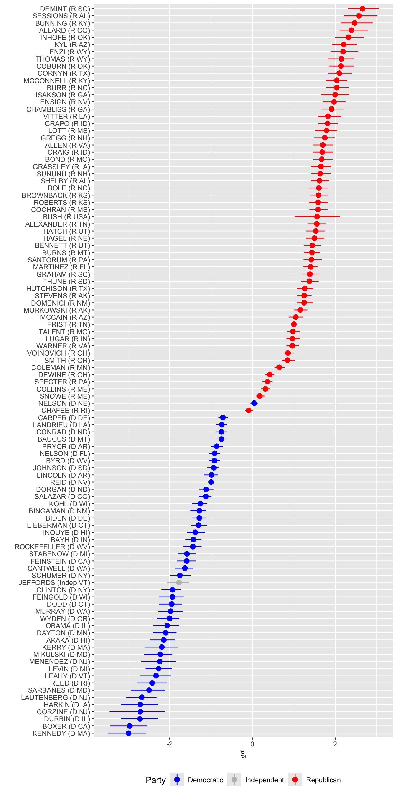
Extract the ideal point data:

Code
legislator_summary_1 <- bind_cols(
  s109_legis_data,
  as_tibble(
    summary(legislators_fit_1, par = "xi")$summary
  )
) |>
  mutate(
    legislator = fct_reorder(legislator, mean)
  )
Code
ggplot(
  legislator_summary_1,
  aes(
    x = legislator,
    y = mean,
    ymin = `2.5%`,
    ymax = `97.5%`,
    colour = party
  )
) +
  geom_pointrange() +
  coord_flip() +
  scale_color_manual(
    values = c(
      Democratic = "blue",
      Independent = "gray",
      Republican = "red"
    )
  ) +
  labs(
    y = expression(xi[i]),
    x = "",
    colour = "Party"
  ) +
  theme(legend.position = "bottom")
Figure 1
Code
legislator_summary_1 |> write_csv("legislators.csv")

References

Poole, Keith T., and Howard Rosenthal. 2001. “D-Nominate After 10 Years: A Comparative Update to Congress: A Political-Economic History of Roll-Call Voting.” Legislative Studies Quarterly 26 (1): 5–29. https://doi.org/10.2307/440401.