Birthdays as Instruments for Catholic School Effects
Labs
Published
July 20, 2025
Overview
In this writeup, the goal is to walk through a third approach (in addition to adjusting for covariates and propensity score weighting) you can take towards tackling the issue of confounding. The following diagram illustrates what we’re hoping to achieve:
We want to estimate the (average) causal effect of Catholic Schooling \(D\) on Post-Grad Earnings \(Y\).
However, there is an unmeasured covariate, Work Ethic \(X\) (a fork relative to \(D \leftarrow X \rightarrow Y\)), which is confounding this effect \(D \rightarrow Y\).
So, as Angrist and Krueger (1991) proposed, we can “work around” this confounding (literally, given how the diagram is set up) by using day of birth relative to school cohort as an instrument:
Since this day of birth has no direct causal relationship with work ethic, and
Has no direct causal relationship with Post-Grad Earnings (only an indirect effect on it through Catholic Schooling \(D\)),
This cohort-relative date of birth can play the same role that a random coin flip plays in the “gold standard” of randomized medical trials!
Under these assumptions (which need to be argued for! And are argued for in Angrist and Krueger (1991)), we can recover the causal effect of \(D\) on \(Y\) via the “classical IV estimator”:
Causal diagram illustrating the role of our proposed instrument \(Z\): a student’s day of birth within the cohort they enter school with. If\(Z\) has (a) no direct causal relationship with Work Ethic (\(X\)) and (b) no direct causal relationship with Post-Grad Earnings \(Y\) (that is, only an indirect effect on it through Catholic Schooling \(D\)), then we can recover the causal effect of Catholic Schooling on Post-Grad Earnings by computing \(\beta_{\text{IV}}^{D \rightarrow Y} = \frac{\text{Cov}[Z,Y]}{\text{Cov}[D,Y]}\)
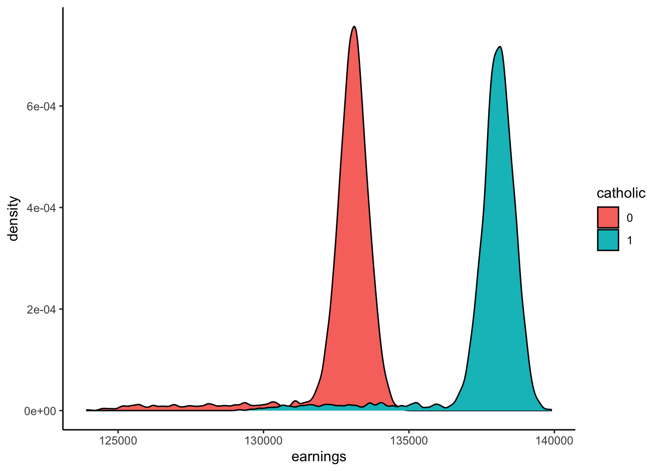
In this writeup, we will generate simulated data on birthdates, school-dropout behavior, and eventual earnings, then use the above IV estimator formula to recover the causal effect of Catholic Schooling on Post-Grad Earnings. We can then verify the accuracy of this estimate, since we generated the data in the first place! The beauty of generative modeling 😉
Uniformly-Distributed Birthdays and Catholic Schooling
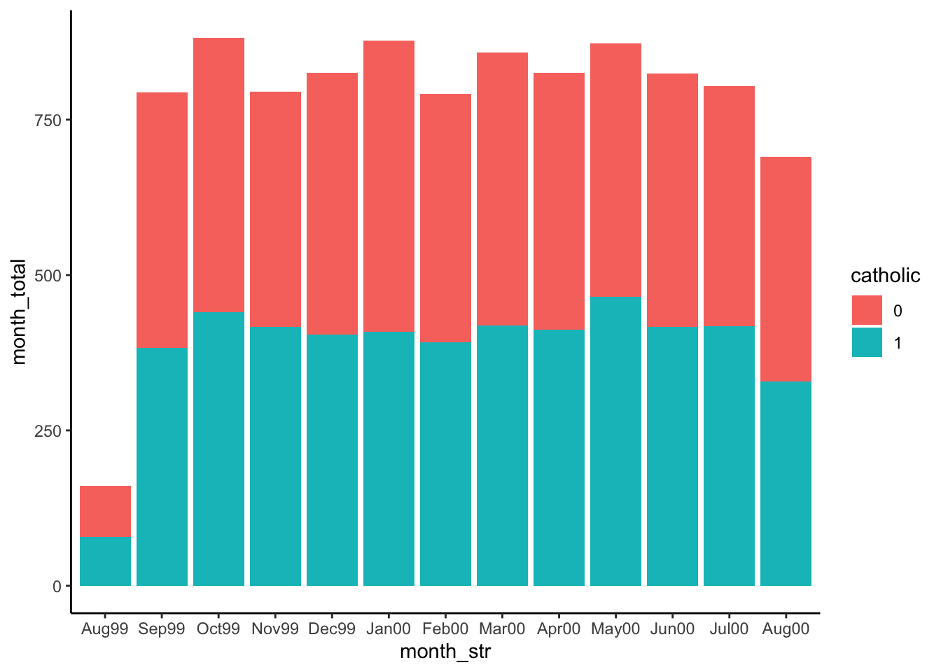
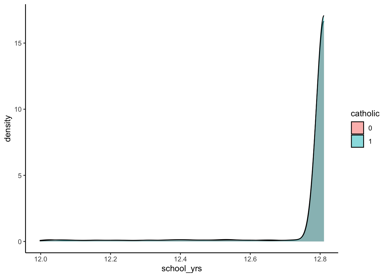
What percentage of students will actually have a chance to drop out? i.e., What proportion of students are born so that they turn 18 before the last day of school?
`summarise()` has regrouped the output.
ℹ Summaries were computed grouped by dob and catholic.
ℹ Output is grouped by dob.
ℹ Use `summarise(.groups = "drop_last")` to silence this message.
ℹ Use `summarise(.by = c(dob, catholic))` for per-operation grouping
  (`?dplyr::dplyr_by`) instead.
`summarise()` has regrouped the output.
ℹ Summaries were computed grouped by month_str and catholic.
ℹ Output is grouped by month_str.
ℹ Use `summarise(.groups = "drop_last")` to silence this message.
ℹ Use `summarise(.by = c(month_str, catholic))` for per-operation grouping
  (`?dplyr::dplyr_by`) instead.
Code
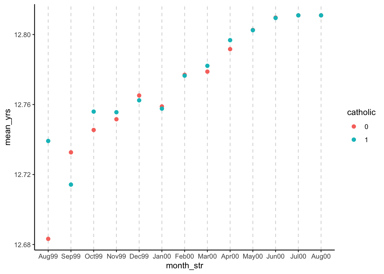
# Plot mean school days by monthschooling_df |>ggplot(aes(x=month_str, y=mean_yrs, color=catholic)) +geom_vline(aes(xintercept=month_str), linetype='dashed', linewidth=0.5, alpha=0.18) +geom_point(size=2) +theme_classic()
Warning: There was 1 warning in `mutate()`.
ℹ In argument: `qtr = case_match(month_str, q1 ~ 1, q2 ~ 2, q3 ~ 3, q4 ~ 4)`.
ℹ In group 1: `month_str = Aug99`.
Caused by warning:
! `case_match()` was deprecated in dplyr 1.2.0.
ℹ Please use `recode_values()` instead.
`summarise()` has regrouped the output.
ℹ Summaries were computed grouped by qtr and catholic.
ℹ Output is grouped by qtr.
ℹ Use `summarise(.groups = "drop_last")` to silence this message.
ℹ Use `summarise(.by = c(qtr, catholic))` for per-operation grouping
  (`?dplyr::dplyr_by`) instead.
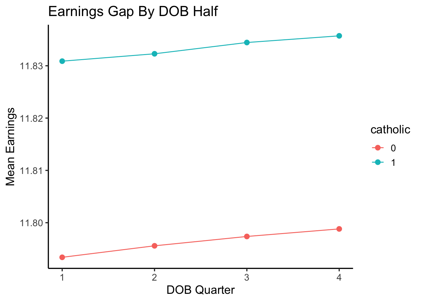
Code
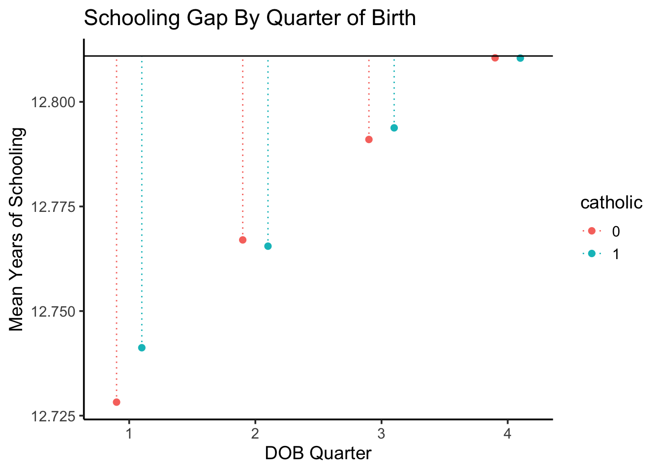
qtr_df |>ggplot(aes(x=qtr, y=mean_yrs_qtr, color=catholic)) +geom_point(stat='identity', size=2, position=position_dodge2(width=0.4) ) +geom_segment(aes(yend=max_schooling),# position=position_jitterdodge(# #dodge.width=0.5# ),position=position_dodge2(width=0.4),linetype='dotted', linewidth=0.5 ) +# ylim(12.759, 12.82) +geom_hline(aes(yintercept=max_schooling,#linetype='Max Possible' ),linewidth=0.5 ) +# scale_linetype_manual("", values=c("dashed")) +# geom_text(x=2.5, y=12.81, label='Maximum Possible (Non-Dropout Amount)', vjust=-1) +labs(title="Schooling Gap By Quarter of Birth",x="DOB Quarter",y="Mean Years of Schooling" ) +theme_classic(base_size=14)
`summarise()` has regrouped the output.
ℹ Summaries were computed grouped by half and catholic.
ℹ Output is grouped by half.
ℹ Use `summarise(.groups = "drop_last")` to silence this message.
ℹ Use `summarise(.by = c(half, catholic))` for per-operation grouping
  (`?dplyr::dplyr_by`) instead.
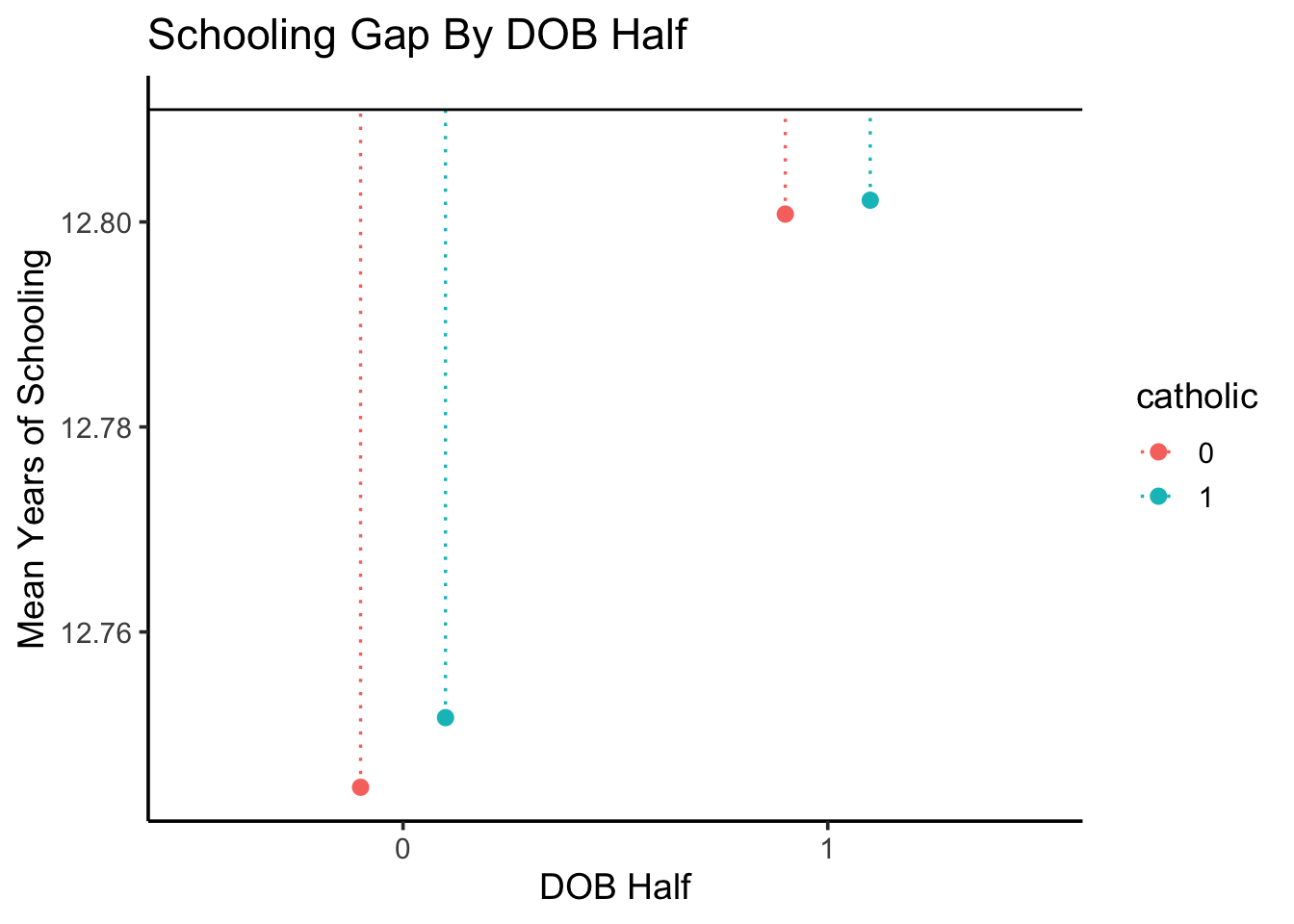
Code
half_df |>ggplot(aes(x=half, y=mean_yrs_half, color=catholic)) +geom_point(stat='identity', size=2.5,position=position_dodge2(width=0.4) ) +geom_segment(aes(yend=max_schooling),position=position_dodge2(width=0.4),linetype='dotted', linewidth=0.6 ) +# ylim(12.759, 12.82) +geom_hline(aes(yintercept=max_schooling,#linetype='Max Possible' ),linewidth=0.5 ) +# scale_linetype_manual("", values=c("dashed")) +# geom_text(x=1.5, y=12.81, label='Maximum Possible (Non-Dropout Amount)', vjust=-1) +labs(title="Schooling Gap By DOB Half",x="DOB Half",y="Mean Years of Schooling" ) +#xlim(0.5, 2.5) +# ylim(12.76, 12.82) +theme_classic(base_size=14)
`summarise()` has regrouped the output.
ℹ Summaries were computed grouped by half and catholic.
ℹ Output is grouped by half.
ℹ Use `summarise(.groups = "drop_last")` to silence this message.
ℹ Use `summarise(.by = c(half, catholic))` for per-operation grouping
  (`?dplyr::dplyr_by`) instead.
`summarise()` has regrouped the output.
ℹ Summaries were computed grouped by qtr and catholic.
ℹ Output is grouped by qtr.
ℹ Use `summarise(.groups = "drop_last")` to silence this message.
ℹ Use `summarise(.by = c(qtr, catholic))` for per-operation grouping
  (`?dplyr::dplyr_by`) instead.
Angrist, Joshua D., and Alan B. Krueger. 1991. “Does Compulsory School Attendance Affect Schooling and Earnings?”The Quarterly Journal of Economics 106 (4): 979–1014. https://doi.org/10.2307/2937954.