import pandas as pd
pop_df = pd.DataFrame({'quote_unquote_race': [0, 1], 'prop_uses_drugs': [0.16, 0.18]})
pop_df| quote_unquote_race | prop_uses_drugs | |
|---|---|---|
| 0 | 0 | 0.16 |
| 1 | 1 | 0.18 |
As an opening disclaimer: recall that we know from statistical theory (e.g., the material that forms the basis of DSAN5100) that, given a population of size \(\nu\) (“nu”, the Greek version of \(n\)), even if we conduct smaller samples of size \(n \ll \nu\), we can infer fairly accurate estimates of some property of the population, especially as \(n \rightarrow \nu\).
So, given that framework, and our goal of laying out operationalization as clearly as possible, you can keep in mind here that:
Studies of drug usage, drawing on a range of anonymized surveys, have slowly started to come up with estimates of population drug usage by self-reported race, which tend to find that the rate of narcotics usage is slightly higher for the white population than for the black population in the US (left panel):

Mathematically, then, let’s start laying out our axioms or antecedents, that we’ll work with in building up descriptive definitions of fairness.
Let \(\overline{\Pi}\) represent the entire population of the US, so that e.g. \(\Pr_{\overline{\Pi}}(E)\) represents the probability that a randomly-chosen person from the population satisfies event \(E\). Let \(\overline{\mathcal{W}}\) and \(\overline{\mathcal{B}}\) represent the white and black populations of the US respectively (recall from e.g. DSAN5100 the use of Greek letters, or at least curly capitalized Latin letters, to represent population parameters! And, as for why they have \(\overline{\text{overlines}}\) above them, read onwards).
Let’s first attempt (and fail) to define a Random Variable \(\widetilde{A}\) (short for “Protected Attribute” in this case) representing the race self-reported to the US Census for a randomly-chosen person from the population of the US (\(\overline{\Pi}\)), such that
\[ \widetilde{A} = \begin{cases} 0 &\text{if Self-Reported White} \\ 1 &\text{if Self-Reported Black} \end{cases} \]
Why is there a tilde (~) above the \(A\) there (and why does this fail to serve as a valid Random Variable as defined in probability theory)? Because, before we can even get off the ground, we have to have the background knowledge that individuals responding to the Census’ questions can list more than one race: there are many individuals in the US for whom the event \(\widetilde{A} = 0\) and \(\widetilde{A} = 1\) both occur if they happen to be the randomly-chosen person. Thus, since Random Variables are by definition:
\(\widetilde{A}\) is straightforwardly not a valid Random Variable—the conditions of the Kolmogorov axioms, which enable expressions in probability theory to be “true” in the same way that the ZFC axioms enable \(1 + 1 = 2\) to be “true”, do not permit non-mutually-exclusive outcomes.
So, if we simply ignore this fact and “jump” directly to white vs. black in the way that this is usually done—a jump that, admittedly, we made ourselves in Question 4 of HW1—this should trigger a “red flag” in your mind, with respect to the question from the Operationalization slides about, “is this variable really measuring what it says it is measuring?”
To address this issue, at minimum, we’ll need to define two Random Variables \(B\) and \(W\), such that
\[ \begin{align*} B &= \begin{cases} 0 &\text{if Did Not Self-Report Black} \\ 1 &\text{if Self-Reported Black} \end{cases} \\ W &= \begin{cases} 0 &\text{if Did Not Self-Report White} \\ 1 &\text{if Self-Reported White} \end{cases} \end{align*} \]
So that now \(B = 1\) and \(W = 1\) can both be true for an individual, which does not violate any Kolmogorov axioms!
Then, we can read more into the methodology that the Hamilton Project/Brookings study cited above uses, to find that they
So, solely for the (descriptive) purpose of matching their provided data on drug usage with base rate information from the Census (see below), we’ll now define a non-tilde version of \(A\) which is what the two bars in the above plots really represent. Letting
\[ S = \begin{cases} 0 &\text{if Multiple Self-Reported Races} \\ 1 &\text{if Single Self-Reported Race} \end{cases} \]
we can now handle the first bullet point by defining a new sub-population \(\Sigma \subset \overline{\Pi}\) consisting of all Census respondents who self-reported only one race, i.e., all Census respondents in \(\overline{\Pi}\) for whom \(S = 1\).
But, to handle the second bullet point, we need to define a second sub-population \(\Pi \subset \Sigma \subset \overline{\Pi}\), of those individuals in \(\Sigma\) for whom \(W = 1\) or \(B = 1\).
It is with respect to this second sub-population \(\Pi\) that we can now finally define a valid binary Random Variable \(A\) as
\[ A = \begin{cases} 0 &\text{if }W = 1 \\ 1 &\text{if }B = 1 \end{cases} \]
where we need to keep in mind that \(A\) is only well-defined with respect to \(\Pi \subset \Sigma \subset \overline{\Pi}\).
Now, as the Hamilton Institute/Brookings study (and many many, probably most, studies of race in the US) defines it implicitly, we can therefore be more explicit here that we are:
Correspondingly, we can map:
I will drop the scare-quotes on “Black” and “White” in a lot of places going forward, so your job is to insert them in your mind when you read the two non-scare-quoted words! I understand if that strikes you as pedantic at first, but please keep in mind the goal of transparency and reproducibility in science (those aren’t even from this class, they’re from the core DSAN5000 class, week 1!): the point is to enable people who are (rightfully) skeptical about data scientists studying race to at least be able to scroll up here and uncover some of the layers of assumptions undergirding our operationalization of “race” here.
Now, to characterize the height of the bar plotted in the figure’s left panel (as opposed to the split of the population into two separate bars), we need to define \(D\) as a Random Variable (short for “Drugs” in this case) representing the drug use of a randomly-chosen person from \(\Pi\), such that
\[ D = \begin{cases} 0 &\text{if Doesn't Use Drugs} \\ 1 &\text{if Uses Drugs} \end{cases} \]
And now we can represent the two bar heights, the two population-level parameters, as:
\[ \begin{align*} \mathbb{E}[D \mid A = 0] = \Pr(D = 1 \mid A = 0) &\approx 0.18 \\ \mathbb{E}[D \mid A = 1] = \Pr(D = 1 \mid A = 1) &\approx 0.16 \end{align*} \]
Where the expectation and probability measures are equal in this case because the Random Variable \(D\) is binary (0/1)[1].
Notice how, there are implementation factors coming into play in moving from this information towards the Fairness in AI material below, since we have a somewhat weird case of something (drug use) that we can infer at the population level despite not being able to easily observe it at the individual level. In other words, to move to the next “step” from this one, we’re already pushing a lot of stuff-from-weeks-1-and-2 (for example, the ethics of elicitation of sensitive data—an individual is not going to be as forthcoming in their illegal drug usage as they would be their eye color).
\[ \mathbb{E}[X] \overset{\text{def}}{=} \sum_{v_X \in \mathcal{R}_X}v_X \cdot \Pr(X = v_X) = 0 \cdot \Pr(X = 0) + 1 \cdot \Pr(X = 1) = \Pr(X = 1) \]
Although the population-level data above is technically available for use by researchers, on its own it doesn’t help very much for researchers working with ML-based classifiers for example, since it basically represents a dataset with \(N = 2\) observations:
import pandas as pd
pop_df = pd.DataFrame({'quote_unquote_race': [0, 1], 'prop_uses_drugs': [0.16, 0.18]})
pop_df| quote_unquote_race | prop_uses_drugs | |
|---|---|---|
| 0 | 0 | 0.16 |
| 1 | 1 | 0.18 |
To even get started in terms of being able to use this data to evaluate fairness, we need to also know the base rates of the two subgroups \(\mathcal{B}\) and \(\mathcal{W}\) with respect to their combined population \(\Sigma\). For example, Chapter 3 of Barocas et al. (2024) builds its description of fairness in AI around classification as the problem of determining (predicting) values of \(y\) for given values of \(x\), rooted in jointly distributed Random Variables \(X\) and \(Y\), with a particular collected dataset viewed as samples from
a probability distribution over pairs of values \((x,y)\) that the random variables \((X,Y)\) might take on.
In our case, notice how we currently only have the two conditional expectations written above, not a full joint distribution of \(D\) and \(A\). So, we should be able to identify the missing piece by writing out the joint distribution as a function of conditional and marginal distributions (in prob/stats textbooks, this is usually introduced as the definition of conditional probability):
\[ \Pr(D \mid A) = \frac{\Pr(D, A)}{\Pr(A)} \implies \Pr(D, A) = \underbrace{\Pr(D \mid A)}_{\text{We have this}}\underbrace{\Pr(A)}_{\text{We don't have this}} \]
So, we have to go out and find the missing term \(\Pr(A)\). Thankfully for this case, the US Census Bureau’s job is to take censuses of the self-reported race of the US population. Less thankfully, these are reported with respect to \(\overline{\Pi}\), not \(\Pi\), so we’ll need to re-normalize.
You can find the Census population percentages here, which tell us that:
First, since the Census provides \(\Pr_{\overline{\Pi}}(S = 0)\), but the Hamilton/Brookings study’s population is those for whom \(S = 1\), we’ll need to use the Kolmogorov axioms to derive
\[ \textstyle \Pr_{\overline{\Pi}}(S = 1) = 1 - \Pr_{\overline{\Pi}}(S = 0) = 0.969. \]
From this quantity we can derive
\[ \begin{align*} \textstyle \Pr_{\overline{\Pi}}(W = 1 \mid S = 1) &= \frac{\Pr_{\overline{\Pi}}(W = 1, S = 1)}{\Pr_{\overline{\Pi}}(S = 1)} = \frac{0.753}{0.969} \approx 0.777 \\ \textstyle \Pr_{\overline{\Pi}}(B = 1 \mid S = 1) &= \frac{\Pr_{\overline{\Pi}}(B = 1, S = 1)}{\Pr_{\overline{\Pi}}(S = 1)} = \frac{0.137}{0.969} \approx 0.141 \\ \end{align*} \]
therefore giving us (by the way we defined \(\Sigma\) above):
\[ \begin{align*} \textstyle \Pr_{\Sigma}(W = 1) &= 0.777 \\ \textstyle \Pr_{\Sigma}(B = 1) &= 0.141 \end{align*} \]
and finally, by the way we defined \(\Pi\) (where, since this is our target population, the one we’d like to use for the remainder of the demo, we define \(\Pr_{\Pi}(E) \equiv \Pr(E)\)),
\[ \begin{align*} \Pr(A = 0) &= \frac{\Pr_{\Sigma}(W = 1)}{\Pr_{\Sigma}(W = 1 \vee B = 1)} = \frac{0.777}{0.777 + 0.141} \approx 0.846 \\ \Pr(A = 1) &= \frac{\Pr_{\Sigma}(B = 1)}{\Pr_{\Sigma}(W = 1 \vee B = 1)} = \frac{0.141}{0.777 + 0.141} \approx 0.154 \end{align*} \]
Now that we have the missing piece allowing us to fully characterize the joint distribution, we can (finally) start deriving a few of the non-immediately-obvious implications from the data we have. For example:
The probability of being a drug user
\[ \begin{align*} \Pr(D = 1) &= \Pr(D = 1, A = 0) + \Pr(D = 1, A = 1) \\ &= \Pr(D = 1 \mid A = 0)\Pr(A = 0) + \Pr(D = 1 \mid A = 1)\Pr(A = 1) \\ &= (0.18)(0.846) + (0.16)(0.154) \approx 0.177 \end{align*} \]
The probability of being a non-drug user (a sanity check to make sure our probabilities satisfy Kolmogorov axioms)
\[ \begin{align*} \Pr(D = 0) &= \Pr(D = 0, A = 0) + \Pr(D = 0, A = 1) \\ &= \Pr(D = 0 \mid A = 0)\Pr(A = 0) + \Pr(D = 0 \mid A = 1)\Pr(A = 1) \\ &= (0.82)(0.846) + (0.84)(0.154) \approx 0.823 \end{align*} \]
The probability that someone is black given that they are a drug user
\[ \begin{align*} \Pr(A = 1 \mid D = 1) &\overset{\text{Bayes}}{\underset{\text{Thm}}{=}} \frac{\Pr(D = 1 \mid A = 1)\Pr(A = 1)}{\Pr(D = 1)} = \frac{(0.16)(0.154)}{0.177} \\ &\approx 0.139 \end{align*} \]
The probability that someone is white given that they are a drug user
\[ \begin{align*} \Pr(A = 0 \mid D = 1) &\overset{\text{Bayes}}{\underset{\text{Thm}}{=}} \frac{\Pr(D = 1 \mid A = 0)\Pr(A = 0)}{\Pr(D = 1)} = \frac{(0.18)(0.846)}{0.177} \\ &\approx 0.860 \end{align*} \]
And, more generally, we can write out the entire joint distribution in a table like
| \(D = 0\) | \(D = 1\) | |
|---|---|---|
| \(A = 0\) | \(\Pr(A = 0, D = 0)\) | \(\Pr(A = 0, D = 1)\) |
| \(A = 1\) | \(\Pr(A = 1, D = 0)\) | \(\Pr(A = 1, D = 1)\) |
Which we compute using Python here to save time (though in general the types of calculations above are fair game for assignments / exams!)
import numpy as np
pA0 = 0.846
pA1 = 1 - pA0 # Hooray for mantissas (...mantissae? mantissi?)
pD1_given_A0 = 0.18
pD0_given_A0 = 1 - pD1_given_A0
pD1_given_A1 = 0.16
pD0_given_A1 = 1 - pD1_given_A1

# Joint probabilities
pD1_A0 = pD1_given_A0 * pA0
print(pD1_A0)
pD1_A1 = pD1_given_A1 * pA1
print(pD1_A1)
pD0_A0 = pD0_given_A0 * pA0
print(pD0_A0)
pD0_A1 = pD0_given_A1 * pA1
print(pD0_A1)

joint_dist = np.array([
    [pD0_A0, pD1_A0],
    [pD0_A1, pD1_A1]
])
print(joint_dist)

print(np.sum(joint_dist))
print(pD0_A0 + pD0_A1 + pD1_A0 + pD1_A1) # Coolio
0.15228
0.024640000000000006
0.69372
0.12936000000000003
[[0.69372 0.15228]
[0.12936 0.02464]]
1.0
1.0Now, moving from 5100-esque to 5450-specific topics, let’s think about a decision-making system which utilizes surveillance cameras installed around a given neighborhood. This system aims to identify people’s faces using these cameras and then, on the basis of a given person \(i\)’s facial image features \(X_i\), classify them into one of two classes:
\[ \widehat{D}_i = \begin{cases} 0 &\text{if }i\textbf{ Not}\text{ a Predicted Drug User} \\ 1 &\text{if }i\textbf{ Is}\text{ a Predicted Drug User} \end{cases} \]
It turns out that, given the descriptive (and context-free) definitions of fairness at the core of the Fairness in AI literature, we have almost everything that we need, besides a loss function.
Using a slightly different notation than the one we use in e.g. DSAN 5300 (we can convert between the two notations if need be!), in a fairness context the loss is often parameterized with respect to a given true label value \(y\) and a given prediction for that label \(\widehat{y}\): \(L(\widehat{y}, y)\) tells us the “badness” of predicting a value \(\widehat{y}\) when the true value that we were trying to predict is \(y\).
One standard loss function, used by pretty much any binary classifier (say, those in scikit-learn) unless the default settings are modified, is the misclassification loss:
\[ L(0, 0) = 0, L(0, 1) = 1, L(1, 0) = 1, L(1, 1) = 0 \]
This loss function assigns a “badness” of 1 when the prediction was incorrect, and a “badness” of 0 when the prediction was correct, so that it can be condensed even more using the indicator function \(\mathbb{1}\) into just:
\[ L(\widehat{y}, y) = \mathbb{1}[\widehat{y} \neq y]. \]
We can also represent this loss function in a form that resembles a confusion matrix (which we’ll use a lot from now on!), keeping in mind that it’s just the same form as a confusion matrix, not a confusion matrix itself:
| \(\widehat{D}_i = 0\) | \(\widehat{D}_i = 1\) | |
|---|---|---|
| \(D = 0\) | 0 | 1 |
| \(D = 1\) | 1 | 0 |
Statistical Independence is satisfied if
\[ \Pr(\widehat{D} = 1 \mid A = 0) = \Pr(\widehat{D} = 1 \mid A = 1) \]
So, let’s see how/whether this fairness definition “matches up with” our intuitions around fairness!
First, let’s construct a “population” of size \(\nu = 1000\) (since our estimates only go to 3 decimal places max), using the joint distribution derived above, that we can sample from (though, for our purposes here, our “sample” will in fact be the entire population, so that \(N = \nu = 1000\)):
import pandas as pd
nu = 1000
pop_df = pd.DataFrame({'A': [0]*nu, 'D': [0]*nu})
pop_df.head()| A | D | |
|---|---|---|
| 0 | 0 | 0 |
| 1 | 0 | 0 |
| 2 | 0 | 0 |
| 3 | 0 | 0 |
| 4 | 0 | 0 |
print(nu * joint_dist)[[693.72 152.28]
[129.36 24.64]]D0_A0_df = pd.DataFrame([{'D': 0, 'A': 0}] * 694) # dist[0,0]
D0_A1_df = pd.DataFrame([{'D': 0, 'A': 1}] * 129) # dist[1,0]
D1_A0_df = pd.DataFrame([{'D': 1, 'A': 0}] * 152) # dist[0,1]
D1_A1_df = pd.DataFrame([{'D': 1, 'A': 1}] * 25) # dist[1,1]
pop_df = pd.concat([D0_A0_df, D0_A1_df, D1_A0_df, D1_A1_df], axis=0, ignore_index=True)
pop_df| D | A | |
|---|---|---|
| 0 | 0 | 0 |
| 1 | 0 | 0 |
| 2 | 0 | 0 |
| 3 | 0 | 0 |
| 4 | 0 | 0 |
| ... | ... | ... |
| 995 | 1 | 1 |
| 996 | 1 | 1 |
| 997 | 1 | 1 |
| 998 | 1 | 1 |
| 999 | 1 | 1 |
1000 rows × 2 columns
len(pop_df[pop_df['D'] == 1])177Now let’s pretend \(X_i\) is some noisy measurement of \(A_i\), train a classifier to predict \(D_i\) from \(X_i\), and see if we get “fairness”!
import numpy as np
rng = np.random.default_rng(seed=5450)
pop_df['X_bin'] = pop_df['A'].apply(lambda x: 1 if x == 1 else -1)
# Random (low chance) flip
pop_df['X_mult'] = rng.choice([1,-1], size=len(pop_df), p=[0.95,0.05])
pop_df['X_result'] = pop_df['X_bin'] * pop_df['X_mult']
pop_df['X_noise'] = rng.normal(0, 0.1, size=len(pop_df))
pop_df['X'] = pop_df['X_result'] + pop_df['X_noise']
pop_df['X_rand'] = rng.normal(0, 0.1, size=len(pop_df))
pop_df| D | A | X_bin | X_mult | X_result | X_noise | X | X_rand | |
|---|---|---|---|---|---|---|---|---|
| 0 | 0 | 0 | -1 | 1 | -1 | -0.054224 | -1.054224 | -0.050844 |
| 1 | 0 | 0 | -1 | 1 | -1 | -0.239642 | -1.239642 | 0.047055 |
| 2 | 0 | 0 | -1 | 1 | -1 | 0.067170 | -0.932830 | -0.010561 |
| 3 | 0 | 0 | -1 | -1 | 1 | 0.120252 | 1.120252 | -0.092252 |
| 4 | 0 | 0 | -1 | 1 | -1 | 0.026217 | -0.973783 | -0.163111 |
| ... | ... | ... | ... | ... | ... | ... | ... | ... |
| 995 | 1 | 1 | 1 | 1 | 1 | 0.072730 | 1.072730 | -0.120465 |
| 996 | 1 | 1 | 1 | 1 | 1 | -0.032165 | 0.967835 | 0.013276 |
| 997 | 1 | 1 | 1 | 1 | 1 | -0.070791 | 0.929209 | 0.006057 |
| 998 | 1 | 1 | 1 | 1 | 1 | 0.060893 | 1.060893 | 0.092034 |
| 999 | 1 | 1 | 1 | 1 | 1 | -0.043217 | 0.956783 | 0.110954 |
1000 rows × 8 columns
black_df = pop_df[pop_df['A'] == 1].copy()
black_df['X'].mean()0.9368364928954515black_df['X'].std()0.37793852152251584white_df = pop_df[pop_df['A'] == 0].copy()
white_df['X'].mean()-0.8899012951427693white_df['X'].std()0.46257415929089934pd.crosstab(pop_df['A'], pop_df['D'], margins=True, normalize=True)| D | 0 | 1 | All |
|---|---|---|---|
| A | |||
| 0 | 0.694 | 0.152 | 0.846 |
| 1 | 0.129 | 0.025 | 0.154 |
| All | 0.823 | 0.177 | 1.000 |
pd.crosstab(pop_df['A'], pop_df['D'], margins=True, normalize='columns')| D | 0 | 1 | All |
|---|---|---|---|
| A | |||
| 0 | 0.843256 | 0.858757 | 0.846 |
| 1 | 0.156744 | 0.141243 | 0.154 |
pd.crosstab(pop_df['A'], pop_df['D'], margins=True, normalize='index')| D | 0 | 1 |
|---|---|---|
| A | ||
| 0 | 0.820331 | 0.179669 |
| 1 | 0.837662 | 0.162338 |
| All | 0.823000 | 0.177000 |
pop_df[['A','D','X']].corr()| A | D | X | |
|---|---|---|---|
| A | 1.000000 | -0.016390 | 0.825867 |
| D | -0.016390 | 1.000000 | -0.037118 |
| X | 0.825867 | -0.037118 | 1.000000 |
import seaborn as sns
sns.boxplot(x='A', y='X', data=pop_df)
sns.boxplot(x='X', y='D', orient='h', data=pop_df)
from sklearn.neural_network import MLPClassifier
from sklearn.svm import LinearSVC
from sklearn.linear_model import LogisticRegression
from sklearn.tree import DecisionTreeClassifier, plot_tree
from sklearn.preprocessing import StandardScaler
scaler = StandardScaler()
from sklearn.metrics import confusion_matrix, roc_curve, RocCurveDisplay, ConfusionMatrixDisplay
from sklearn.model_selection import train_test_split
#clf = LinearSVC()
#clf = MLPClassifier(hidden_layer_sizes=(10,10), activation='logistic')
clf = LogisticRegression()
#clf = DecisionTreeClassifier(max_depth=1)X_df = pop_df[['X','X_rand']].copy()
X_scaled = scaler.fit_transform(X_df)
d_df = pop_df['D'].copy()
X_train, X_test, d_train, d_test = train_test_split(X_scaled, d_df)
clf = clf.fit(X_train, d_train)X_trainarray([[ 2.01620819, -1.32996031],
[ 2.2518996 , -0.75840806],
[ 2.14098014, 0.31504902],
...,
[-0.28251252, 1.00551134],
[-0.57882442, -0.15290433],
[ 1.99170214, 0.46089925]])X_df.shape, d_df.shape((1000, 2), (1000,))d_test_hat = clf.predict(X_test)confusion_matrix(d_test, d_test_hat)array([[207, 0],
[ 43, 0]])pop_df['D_hat'] = clf.predict(pop_df[['X','X_rand']])
pop_df/usr/local/lib/python3.11/dist-packages/sklearn/utils/validation.py:2732: UserWarning: X has feature names, but LogisticRegression was fitted without feature names
warnings.warn(| D | A | X_bin | X_mult | X_result | X_noise | X | X_rand | D_hat | |
|---|---|---|---|---|---|---|---|---|---|
| 0 | 0 | 0 | -1 | 1 | -1 | -0.054224 | -1.054224 | -0.050844 | 0 |
| 1 | 0 | 0 | -1 | 1 | -1 | -0.239642 | -1.239642 | 0.047055 | 0 |
| 2 | 0 | 0 | -1 | 1 | -1 | 0.067170 | -0.932830 | -0.010561 | 0 |
| 3 | 0 | 0 | -1 | -1 | 1 | 0.120252 | 1.120252 | -0.092252 | 0 |
| 4 | 0 | 0 | -1 | 1 | -1 | 0.026217 | -0.973783 | -0.163111 | 0 |
| ... | ... | ... | ... | ... | ... | ... | ... | ... | ... |
| 995 | 1 | 1 | 1 | 1 | 1 | 0.072730 | 1.072730 | -0.120465 | 0 |
| 996 | 1 | 1 | 1 | 1 | 1 | -0.032165 | 0.967835 | 0.013276 | 0 |
| 997 | 1 | 1 | 1 | 1 | 1 | -0.070791 | 0.929209 | 0.006057 | 0 |
| 998 | 1 | 1 | 1 | 1 | 1 | 0.060893 | 1.060893 | 0.092034 | 0 |
| 999 | 1 | 1 | 1 | 1 | 1 | -0.043217 | 0.956783 | 0.110954 | 0 |
1000 rows × 9 columns
if isinstance(clf, DecisionTreeClassifier):
  plot_tree(clf)
test_X0 = np.arange(-1, 1, 0.1)
test_Xrand = rng.normal(0, 0.1, size=len(test_X0))
test_Xmat = np.column_stack([test_X0, test_Xrand])
test_Xmatarray([[-1.00000000e+00, -8.21496502e-02],
[-9.00000000e-01, -1.18804351e-01],
[-8.00000000e-01, -9.71993639e-02],
[-7.00000000e-01, 1.79121572e-01],
[-6.00000000e-01, 7.54615529e-02],
[-5.00000000e-01, -7.55314281e-02],
[-4.00000000e-01, -2.14828193e-02],
[-3.00000000e-01, -5.39771961e-02],
[-2.00000000e-01, -1.24518105e-01],
[-1.00000000e-01, 1.15651561e-01],
[-2.22044605e-16, -1.11209055e-01],
[ 1.00000000e-01, -1.63469797e-01],
[ 2.00000000e-01, -4.00110245e-02],
[ 3.00000000e-01, -8.82016598e-02],
[ 4.00000000e-01, -2.74525280e-02],
[ 5.00000000e-01, -5.04958858e-02],
[ 6.00000000e-01, -3.54260686e-02],
[ 7.00000000e-01, 4.46857290e-03],
[ 8.00000000e-01, -1.21658993e-01],
[ 9.00000000e-01, -3.37236460e-02]])clf.predict(test_Xmat)array([0, 0, 0, 0, 0, 0, 0, 0, 0, 0, 0, 0, 0, 0, 0, 0, 0, 0, 0, 0])test_Xmat_pred = clf.predict_proba(test_Xmat)
test_Xmat_predarray([[0.811287 , 0.188713 ],
[0.81442558, 0.18557442],
[0.81643575, 0.18356425],
[0.81365365, 0.18634635],
[0.81801088, 0.18198912],
[0.82315069, 0.17684931],
[0.82450109, 0.17549891],
[0.82739245, 0.17260755],
[0.83091462, 0.16908538],
[0.82894698, 0.17105302],
[0.83514931, 0.16485069],
[0.83823475, 0.16176525],
[0.83832092, 0.16167908],
[0.84129042, 0.15870958],
[0.84241775, 0.15758225],
[0.84491479, 0.15508521],
[0.84676281, 0.15323719],
[0.84819397, 0.15180603],
[0.85224427, 0.14775573],
[0.85288184, 0.14711816]])test_d_prob = test_Xmat_pred[:,1]
test_d_probarray([0.188713 , 0.18557442, 0.18356425, 0.18634635, 0.18198912,
0.17684931, 0.17549891, 0.17260755, 0.16908538, 0.17105302,
0.16485069, 0.16176525, 0.16167908, 0.15870958, 0.15758225,
0.15508521, 0.15323719, 0.15180603, 0.14775573, 0.14711816])def classify(cur_clf, test_Xmat, d_prob_thresh = 0.17):
test_Xmat_pred = cur_clf.predict_proba(test_Xmat)
test_d_prob = test_Xmat_pred[:,1]
test_d_class = np.where(test_d_prob > d_prob_thresh, 1, 0)
return test_d_classtest_d_pred = classify(test_Xmat)
test_d_predarray([1, 1, 1, 1, 1, 1, 1, 1, 0, 1, 0, 0, 0, 0, 0, 0, 0, 0, 0, 0])test_d_true = np.where(test_Xmat[:,0] < 0, 1, 0)
test_d_truearray([1, 1, 1, 1, 1, 1, 1, 1, 1, 1, 1, 0, 0, 0, 0, 0, 0, 0, 0, 0])#RocCurveDisplay.from_estimator(clf, X_test, d_test, plot_chance_level=True)RocCurveDisplay.from_predictions(test_d_true, test_d_pred, plot_chance_level=True)
new_samp_df = pop_df.sample(100, random_state=5450)new_samp_df| D | A | X_bin | X_mult | X_result | X_noise | X | X_rand | |
|---|---|---|---|---|---|---|---|---|
| 899 | 1 | 0 | -1 | 1 | -1 | -0.033770 | -1.033770 | -0.026273 |
| 699 | 0 | 1 | 1 | 1 | 1 | -0.181455 | 0.818545 | -0.023939 |
| 481 | 0 | 0 | -1 | 1 | -1 | -0.200307 | -1.200307 | 0.113340 |
| 503 | 0 | 0 | -1 | 1 | -1 | 0.034218 | -0.965782 | -0.048357 |
| 856 | 1 | 0 | -1 | 1 | -1 | 0.103965 | -0.896035 | 0.015975 |
| ... | ... | ... | ... | ... | ... | ... | ... | ... |
| 896 | 1 | 0 | -1 | 1 | -1 | -0.018532 | -1.018532 | -0.049717 |
| 500 | 0 | 0 | -1 | 1 | -1 | 0.010933 | -0.989067 | 0.030974 |
| 558 | 0 | 0 | -1 | 1 | -1 | -0.001991 | -1.001991 | -0.110632 |
| 414 | 0 | 0 | -1 | 1 | -1 | 0.067946 | -0.932054 | -0.124212 |
| 279 | 0 | 0 | -1 | 1 | -1 | -0.120680 | -1.120680 | -0.015748 |
100 rows × 8 columns
new_test_Xmat = new_samp_df[['X','X_rand']].copy()new_test_preds = classify(new_test_Xmat)/usr/local/lib/python3.11/dist-packages/sklearn/utils/validation.py:2732: UserWarning: X has feature names, but LogisticRegression was fitted without feature names
warnings.warn(confusion_matrix(new_test_preds, new_samp_df['D'])array([[14, 5],
[63, 18]])Fairness comes from the confusion matrix using A instead of D!
confusion_matrix(new_test_preds, new_samp_df['A'])array([[ 8, 11],
[79, 2]])ConfusionMatrixDisplay.from_predictions(new_samp_df['A'], new_test_preds) #, display_labels=['not_drug_user','drug_user'])
confusion_matrix(new_samp_df['A'], new_test_preds, normalize='true')array([[0.09195402, 0.90804598],
[0.84615385, 0.15384615]])Now, if we re-do everything above but with drug usage rates operationalized using arrest rates, we instead have
\[ \begin{align*} \Pr(D = 1 \mid A = 0) &= 0.0040 \\ \Pr(D = 1 \mid A = 1) &= 0.0105 \end{align*} \]
def gen_noisy_feature(pop_race_vec):
  X_bin = pop_df['A'].apply(lambda x: 1 if x == 1 else -1)
  # Random (low chance) flip
  X_mult = rng.choice([1,-1], size=len(pop_race_vec), p=[0.95,0.05])
  X_result = X_bin * X_mult
  X_noise = rng.normal(0, 0.1, size=len(pop_df))
  X_final = X_result + X_noise
  return X_final

def gen_random_feature(pop_race_vec):
  X_rand = rng.normal(0, 0.1, size=len(pop_race_vec))
  return X_rand

def classify(test_Xmat, d_prob_thresh = 0.17):
  test_Xmat_pred = clf.predict_proba(test_Xmat)
  test_d_prob = test_Xmat_pred[:,1]
  test_d_class = np.where(test_d_prob > d_prob_thresh, 1, 0)
  return test_d_class

def construct_population(pD1_given_A0, pD1_given_A1, nu=1000):
  pA0 = 0.846
  pA1 = 1 - pA0
  pD0_given_A0 = 1 - pD1_given_A0
  pD0_given_A1 = 1 - pD1_given_A1
  # Joint probabilities
  pD1_A0 = pD1_given_A0 * pA0
  #print(pD1_A0)
  pD1_A1 = pD1_given_A1 * pA1
  #print(pD1_A1)
  pD0_A0 = pD0_given_A0 * pA0
  #print(pD0_A0)
  pD0_A1 = pD0_given_A1 * pA1
  #print(pD0_A1)
  joint_dist = np.array([
      [pD0_A0, pD1_A0],
      [pD0_A1, pD1_A1]
  ])
  print(joint_dist)
  nu = 1000
  pop_df = pd.DataFrame({'A': [0]*nu, 'D': [0]*nu})
  joint_freqs = nu * joint_dist
  D0_A0_df = pd.DataFrame([{'D': 0, 'A': 0}] * round(joint_freqs[0,0]))
  D0_A1_df = pd.DataFrame([{'D': 0, 'A': 1}] * round(joint_freqs[1,0]))
  D1_A0_df = pd.DataFrame([{'D': 1, 'A': 0}] * round(joint_freqs[0,1]))
  D1_A1_df = pd.DataFrame([{'D': 1, 'A': 1}] * round(joint_freqs[1,1]))
  pop_df = pd.concat([D0_A0_df, D0_A1_df, D1_A0_df, D1_A1_df], axis=0, ignore_index=True)
  #display(pop_df)
  pop_df['X0'] = gen_noisy_feature(pop_df['A'])
  pop_df['X1'] = gen_random_feature(pop_df['A'])
  return pop_df

arrest_df = construct_population(0.0040, 0.0105)
display(arrest_df)
[[0.842616 0.003384]
[0.152383 0.001617]]| D | A | X0 | X1 | |
|---|---|---|---|---|
| 0 | 0 | 0 | -0.971645 | -0.024211 |
| 1 | 0 | 0 | -1.176896 | 0.039959 |
| 2 | 0 | 0 | -1.008070 | -0.026912 |
| 3 | 0 | 0 | -0.999462 | 0.021601 |
| 4 | 0 | 0 | -0.944086 | -0.149199 |
| ... | ... | ... | ... | ... |
| 995 | 1 | 0 | 0.925104 | -0.033928 |
| 996 | 1 | 0 | 1.013372 | -0.130119 |
| 997 | 1 | 0 | 0.898179 | 0.108746 |
| 998 | 1 | 1 | 0.887125 | -0.123374 |
| 999 | 1 | 1 | 0.848386 | -0.082399 |
1000 rows × 4 columns
# Classify
def thresh_classify(cur_clf, test_Xmat, d_prob_thresh = 0.17):
  test_Xmat_pred = cur_clf.predict_proba(test_Xmat)
  test_d_prob = test_Xmat_pred[:,1]
  test_d_class = np.where(test_d_prob > d_prob_thresh, 1, 0)
  return test_d_class

pop_clf = LogisticRegression()
X_pop = arrest_df[['X0','X1']].copy()
d_pop = arrest_df['D'].copy()
pop_clf.fit(X_pop, d_pop)
optimal_pr_d_hat = thresh_classify(pop_clf, X_pop, 0.5)
fair_pr_d_hat = thresh_classify(pop_clf, X_pop, 0.03)
unfair_pr_d_hat = thresh_classify(pop_clf, X_pop, 0.025)
def display_confusion(race_vec, classification_vec):
return ConfusionMatrixDisplay.from_predictions(race_vec, classification_vec) #, display_labels=['not_drug_user','drug_user'])
def display_confusion_normalized(race_vec, classification_vec):
return ConfusionMatrixDisplay.from_predictions(race_vec, classification_vec, normalize='true') #, display_labels=['not_drug_user','drug_user'])For optimal classifier:
display_confusion(arrest_df['A'], optimal_pr_d_hat)
display_confusion_normalized(arrest_df['A'], optimal_pr_d_hat)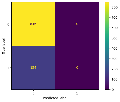
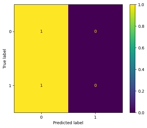
For effective threshold classifier:
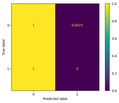
display_confusion(arrest_df['A'], fair_pr_d_hat)
display_confusion_normalized(arrest_df['A'], fair_pr_d_hat)

def compute_unfairness(race_vec, d_hat):
  cmat = confusion_matrix(race_vec, d_hat, normalize='true')
  pr_DH1_A0 = cmat[0,1]
  pr_DH1_A1 = cmat[1,1]
  return abs(pr_DH1_A1 - pr_DH1_A0)

def compute_accuracy(d_vec, d_hat):
  cmat = confusion_matrix(d_vec, d_hat, normalize='all')
  pr_DH0_H0 = cmat[0,0]
  pr_DH1_H1 = cmat[1,1]
  return pr_DH0_H0 + pr_DH1_H1

print(compute_unfairness(arrest_df['A'], fair_pr_d_hat))
print(compute_accuracy(arrest_df['D'], fair_pr_d_hat))
0.002364066193853428
0.993
thresh_vals_macro = np.arange(0, 0.04, 0.0001)
def gen_unfairness_curve(thresh_vals):
  unfairness_data = []

  for cur_thresh in thresh_vals:
    cur_pr_d_hat = thresh_classify(pop_clf, X_pop, cur_thresh)
    cur_unfairness = compute_unfairness(arrest_df['A'], cur_pr_d_hat)
    cur_accuracy = compute_accuracy(arrest_df['D'], cur_pr_d_hat)
    cur_data = {
        'thresh': cur_thresh,
        'unfairness': 10*cur_unfairness,
        'accuracy': cur_accuracy,
    }
    unfairness_data.append(cur_data)
  unfairness_df = pd.DataFrame(unfairness_data)
  return unfairness_df

unfairness_macro_df = gen_unfairness_curve(thresh_vals_macro)unfairness_macro_df| thresh | unfairness | accuracy | |
|---|---|---|---|
| 0 | 0.0000 | 0.0 | 0.005 |
| 1 | 0.0001 | 0.0 | 0.005 |
| 2 | 0.0002 | 0.0 | 0.005 |
| 3 | 0.0003 | 0.0 | 0.005 |
| 4 | 0.0004 | 0.0 | 0.005 |
| ... | ... | ... | ... |
| 395 | 0.0395 | 0.0 | 0.995 |
| 396 | 0.0396 | 0.0 | 0.995 |
| 397 | 0.0397 | 0.0 | 0.995 |
| 398 | 0.0398 | 0.0 | 0.995 |
| 399 | 0.0399 | 0.0 | 0.995 |
400 rows × 3 columns
unfairness_macro_df.plot(x='thresh', y=['unfairness','accuracy'])
thresh_vals_micro = np.arange(0, 0.005, 0.00001)
unfairness_micro_df = gen_unfairness_curve(thresh_vals_micro)
unfairness_micro_df.plot(x='thresh', y=['unfairness','accuracy'])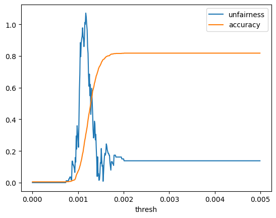
Building on Statistical Parity, Predictive Parity incorporates the actual accuracy of the predictions, requiring only that the rate of correct predictions is equal for \(A = 0\) and \(A = 1\):
\[ \Pr(D = 1 \mid \widehat{D} = 1, A = 0) = \Pr(D = 1 \mid \widehat{D} = 1, A = 1) \]
For any given estimation “score” \(s(X)\) used by the algorithm as a proxy for estimating \(\widehat{\Pr}(D = 1)\)[2], which in turns gets used (e.g., via thresholding) to generate a final prediction \(\widehat{D}\), the probability of using drugs \(\Pr(D = 1)\) is equal for \(A = 0\) and \(A = 1\):
\[ \Pr(D = 1 \mid s(X) = s, A = 0) = \Pr(D = 1 \mid s(X) = s, A = 1), \; \forall s \in [0, 1] \]
This measure is the least bamboozling in the sense that it directly addresses the underlying “risk scores” which, if a given machine learning algorithm does not directly compute itself, can at least be inferred by treating the algorithm like a “black box”.