Week 6: Regularization for Model Selection

DSAN 5300: Statistical Learning
Spring 2025, Georgetown University

Class Sessions

Author

Affiliation

Jeff Jacobs

jj1088@georgetown.edu

Published

Tuesday, February 18, 2025

Open slides in new tab →

Schedule

Today’s Planned Schedule:

	Start	End	Topic
Lecture	6:30pm	7:00pm	Extended Recap / Clarification →
	7:00pm	7:20pm	“Manual” Model Selection: Subsets →
	7:20pm	7:40pm	Key Regularization Building Block: \(L^p\) Norm →
	7:40pm	8:00pm	Regularized Regression Intro →
Break!	8:00pm	8:10pm
	8:10pm	8:50pm	Basically Lasso is the Coolest Thing Ever →
	8:50pm	9:00pm	Scary-Looking But Actually-Fun W07 Preview →

Roadmap

[Week 4] Oh no! When we go beyond linear models, we have to worry about overfitting!
- \(\implies\) New goal! Maximize generalizability rather than accuracy
- \(\implies\) Evaluate models on unseen test data rather than training data
[Week 5] Cross-Validation (CV) as a tool for Model Assessment: For more complex, non-linear models, is there some way we can try to… “foresee” how well a trained model will generalize?
- Answer: Yes! Cross-validation!
[Week 6] Regularization as a tool for Model Selection: Now that we have a method (CV) for imperfectly measuring “generalizability”, is there some way we can try to… allow models to optimize CV but penalize them for unnecessary complexity?
- Answer: Yes! Regularization methods like LASSO and Elastic Net!

[Reminder (W04)] New Goal: Generalizability

Goal 2.0: Statistical Learning

Find…

A function \(\widehat{y} = f(x)\) ✅
That best predicts \(Y\) for given values of \(X\) ✅
For data that has not yet been observed! 😳❓

Clarification: Target Diagrams

Figure 1: Adapted from Fortmann-Roe (2012), “Understanding the Bias-Variance Tradeoff”

Why Was This Helpful for 5100?

Law of Large Numbers:
- Avg(many sample means \(s\)) \(\leadsto\) true mean \(\mu\)
\(\widehat{\theta}\) unbiased estimator for \(\theta\):
- Avg(Estimates \(\widehat{\theta}\)) \(\leadsto\) true \(\theta\)

Relevance for CV Error

In Goal 2.0 world, we choose models on the basis of estimated test error (before, with Goal 1.0, we only used e.g. MSE, RSS, \(R^2\), which was fine for linear regression)
Data \(\mathbf{D}\) = single realization of DGP (for 5300, only relevance is why we don’t look at test set)
\(\left[ \mathbf{D}_{\text{Train}} \middle| \mathbf{D}_{\text{Test}} \right]\) = random permutation of \(\mathbf{D}\)
Bullseye on target = true test error
(We could compute this, but then we’d have to end the study, collect more data… better alternative on next slide!)
Darts thrown around bullseye = estimated test errors (CV fold errors!)
- They don’t hit bullseye because we’re inferring DGP from from sample
True test error = \(f(\mathbf{D}) = f\left( \left[ \mathbf{D}_{\text{Train}} \middle| \mathbf{D}_{\text{Test}} \right] \right)\)
Validation error = \(f(\mathbf{D}_{\text{Train}}) = f\left( \left[ \mathbf{D}_{\text{SubTr}} \middle| \mathbf{D}_{\text{Val}} \right] \right)\),
- \(\implies\) Validation error is an estimate, using a smaller sample \(\mathbf{D}_{\text{Train}}\) drawn from the same distribution (DGP) as true test error!

True Test Error vs. CV Error

Note the icons! Test set = Lake monster: pulling out of water to evaluate kills it 😵

True Test Error \(\varepsilon_{\text{Test}} = \text{Err}_{\text{Test}}\)

Data \(\mathbf{D}\) “arises” out of (unobservable) DGP

Randomly chop \(\mathbf{D}\) into \(\left[ \mathbf{D}_{\text{Train}} \mid \mathbf{D}_{\text{Test}} \right]\)

\(\underbrace{\text{Err}_{\text{Test}}}_{\substack{\text{Test error,} \\ \text{no cap}}} = f(\mathbf{D}_{\text{Train}} \overset{\text{fit}}{\longrightarrow} \underbrace{\mathcal{M}_{\theta} \overset{\text{eval}}{\longrightarrow} \mathbf{D}_{\text{Test}}}_{\text{This kills monster 😢}})\)

Issue: can only be evaluated once, ever 😱

Validation Set Error \(\varepsilon_{\text{Val}} = \widehat{\varepsilon}_{\text{Test}} = \widehat{\text{Err}}_{\text{Test}}\)

\(\text{DGP} \rightarrow \mathbf{D}\); Randomly chop into \([\mathbf{D}_{\text{Train}} \mid \mathbf{D}_{\text{Test}}]\)

Leave \(\mathbf{D}_{\text{Test}}\) alone until end of study

Randomly chop \(\mathbf{D}_{\text{Train}}\) into \([\mathbf{D}_{\text{SubTr}} \mid \mathbf{D}_{\text{Val}}]\)

\(\underbrace{\widehat{\text{Err}}_{\text{Test}}}_{\substack{\text{Test error,} \\ \text{capping a bit}}} = f(\mathbf{D}_{\text{SubTr}} \overset{\text{fit}}{\longrightarrow} \underbrace{\mathcal{M}_{\theta} \overset{\text{eval}}{\longrightarrow} \mathbf{D}_{\text{Val}}}_{\text{Monster still alive!}})\)

\(K\)-Fold Cross-Validation Error \(\varepsilon_{(K)} = \widehat{\varepsilon}_{\text{Test}} = \widehat{\text{E}}\text{rr}_{\text{Test}}\)

\(\text{DGP} \rightarrow \mathbf{D}\); Randomly chop into \([\mathbf{D}_{\text{Train}} \mid \mathbf{D}_{\text{Test}}]\); Leave \(\mathbf{D}_{\text{Test}}\) for end of study

Randomly chop \(\mathbf{D}_{\text{Train}}\) into \(\left[ \mathbf{D}_{\text{TrFold}}^{(1)} \middle| \mathbf{D}_{\text{TrFold}}^{(2)} \middle| \cdots \middle| \mathbf{D}_{\text{TrFold}}^{(K)} \right]\)

For \(i \in \{1, \ldots, K\}\):

\(\varepsilon_{\text{ValFold}}^{(i)} = f\left( \mathbf{D}_{\text{TrFold}}^{(-i)} \overset{\text{fit}}{\longrightarrow} \mathcal{M}_{\theta} \overset{\text{eval}}{\longrightarrow} \mathbf{D}_{\text{TrFold}}^{(i)} \right)\)

\(\underbrace{\widehat{\text{E}}\text{rr}_{\text{Test}}}_{\substack{\text{Test error,} \\ \text{less cap!}}} = \boxed{\frac{1}{K}\sum_{i=1}^{K}\varepsilon^{(i)}_{\text{ValFold}}}~\) (…monster still alive, even after all that!)

General Issue with CV: It’s… Halfway There

CV plots will often look like (complexity on \(x\)-axis and CV error on \(y\)-axis):

Code

library(tidyverse) |> suppressPackageStartupMessages()
library(latex2exp) |> suppressPackageStartupMessages()
cpl_label <- TeX("$M_0$")
sim1k_delta_df <- tibble(
    complexity=1:7,
    cv_err=c(8, 2, 1, 1, 1, 1, 2),
    label=c("","",TeX("$M_3$"),"","",TeX("$M_6$"),"")
)
sim1k_delta_df |> ggplot(aes(x=complexity, y=cv_err, label=label)) +
  geom_line(linewidth=1) +
  geom_point(size=(2/3)*g_pointsize) +
  geom_text(vjust=-0.7, size=10, parse=TRUE) +
  scale_x_continuous(
    breaks=seq(from=1,to=7,by=1)
  ) +
  theme_dsan(base_size=22) +
  labs(
    title="Generic CV Error Plot",
    x = "Complexity",
    y = "CV Error"
  )

We “know” \(\mathcal{M}_3\) preferable to \(\mathcal{M}_6\) (same error yet, less overfitting) \(\implies\) “1SE rule”
But… heuristic \(\;\nimplies\) optimal! What are we gaining/losing as we move \(\mathcal{M}_6 \rightarrow \mathcal{M}_3\)?
Enter REGULARIZATION!

CV Now Goes Into Your Toolbox

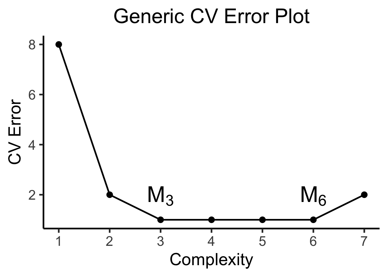
(We will take it back out later, I promise!)

Model Selection

[Week 5 ✅] We have a metric (CV error) for evaluating different models w.r.t. Goal 2.0…
[Week 6 so far] It gets us halfway to what we want, by showing us a “basin” of models with low CV error
[Now] Statistically-principled approach to overfitting that
- Shows us why the 1SE rule “works”
- Quantifies tradeoff: if I only have enough data to estimate \(\beta_j\) for \(J_0 < J\) feats, which \(J_0\) should I choose?

Optimal but Infeasible: Best Subset Selection

Algorithm: Best Subset Selection

Let \(\mathcal{M}^*_0\) be null model: Predicts \(\widehat{y}(x_i) = \overline{y}\) for any \(x_i\)

For \(k = 1, 2, \ldots, J\):

Fit all \(\binom{J}{k}\) possible models with \(k\) predictors, \(\mathcal{M}^*_k\) is model with lowest RSS

Choose from \(\mathcal{M}^*_0, \ldots, \mathcal{M}^*_J\) using CV or heuristics: AIC, BIC, adjusted \(R^2\)

Feasible but Suboptimal: Stepwise Selection

Algorithm: Forward Stepwise Selection

Let \(\mathcal{M}_0\) be null model: Predicts \(\widehat{y}(x_i) = \overline{y}\) for any \(x_i\)

For \(k = 0, 1, \ldots, J - 1\):

Fit \(J - k\) models, each adds single feature to \(\mathcal{M}_k\); call “best” model \(\mathcal{M}_{k+1}\)

Choose from \(\mathcal{M}_0, \ldots, \mathcal{M}_J\) using CV error (or heuristics: AIC, BIC, adjusted \(R^2\))

Algorithm: Backward Stepwise Selection

Let \(\mathcal{M}_J\) be full model: Contains all features

For \(k = J, J - 1, \ldots, 1\):

Fit \(k\) models, each removes single feature from \(\mathcal{M}_k\); call “best” model \(\mathcal{M}_{k-1}\)

Choose from \(\mathcal{M}_0, \ldots, \mathcal{M}_J\) using CV error (or heuristics: AIC, BIC, adjusted \(R^2\))

Stepwise Selection Algorithms are Greedy

Like a mouse who chases closest cheese \(\neq\) path with most cheese
Can get “trapped” in sub-optimal model, if (e.g.) feature is in \(\mathcal{M}^*_4\) but not in \(\mathcal{M}^*_1, \mathcal{M}^*_2, \mathcal{M}^*_3\)!

\(k\)	\(\mathcal{M}^*_k\) (Best Subset)	\(\mathcal{M}_k\) (Forward Stepwise)
1	`rating`	`rating`
2	`rating`, `income`	`rating`, `income`
3	`rating`, `income`, `student`	`rating`, `income`, `student`
4	`cards`, `income`, `student`, `limit`	`rating`, `income`, `student`, `limit`

Regularization for Automatic Model Selection

Ridge Regression
Lasso
Elastic Net

Key Building Block: \(L^p\) Norms

Technically you have seen these before: distance metrics!

\[ \textsf{sim}(\mathbf{u}, \mathbf{v}) \triangleq \underbrace{\| \mathbf{v} - \mathbf{u} \|_p}_{L^p\text{ norm of }\mathbf{u} - \mathbf{v}} = \left( \sum_{i=1}^{n} |v_i - u_i|^p \right)^{1/p} \]

\(\implies\) Euclidean distance is \(L^2\) norm: if \(\mathbf{u} = (0,0)\) and \(\mathbf{v} = (3,4)\),

\[ \| \mathbf{v} - \mathbf{u} \|_2 = \left( |3-0|^2 + |4-0|^2 \right)^{1/2} = 25^{1/2} = \sqrt{25} = 5 \]

We’ll use even simpler form: distance of coefficients \(\boldsymbol\beta\) from zero (so, \(\mathbf{u} = \vec{\mathbf{0}}\))

\[ \| \boldsymbol\beta \|_p = \left( \sum_{j=1}^{J} |\beta_j|^p \right)^{1/p} \]

\(L^1\) and \(L^2\) Norms

\(L^1\) norm has a nice closed form expression as a sum (efficient, vectorizable!):

\[ \| \boldsymbol\beta \|_1 = \left( \sum_{j=1}^{J}|\beta_j|^1 \right)^{1/1} = \boxed{\sum_{j=1}^{J}|\beta_j|} \]

\(L^2\) norm almost a similarly nice expression, besides this zigzag line thing (\(\sqrt{~}\))

\[ \| \boldsymbol\beta \|_2 = \left( \sum_{j=1}^{J}|\beta_j|^2 \right)^{1/2} = \sqrt{\sum_{j=1}^{J}\beta_j^2} \; \; 🤨 \]

Can always convert bound on true Euclidean distance like \(\| \boldsymbol\beta \|_2 \leq 10\) into bound on squared Euclidean distance like \(\| \boldsymbol\beta \|_2^2 \leq 100\). Hence we’ll use squared \(L^p\) norm:

\[ \| \boldsymbol\beta \|_2^2 = \left( \left( \sum_{j=1}^{J}|\beta_j|^p \right)^{1/2} \right)^{2} = \boxed{\sum_{j=1}^{J}\beta_j^2} \; \; 💆 \]

Different Norms \(\leftrightarrow\) Different Distances from \(\vec{\mathbf{0}}\)

Unit Disk in \(L^2\): All points \(\mathbf{v} = (v_x,v_y) \in \mathbb{R}^2\) such that

\[ \| \mathbf{v} \|_2 \leq 1 \iff \| \mathbf{v} \|_2^2 \leq 1 \]

Unit Disk in \(L^1\): All points \(\mathbf{v} = (v_x, v_y) \in \mathbf{R}^2\) such that

\[ \| \mathbf{v} \|_1 \leq 1 \]

Regularized Regression (Finally!)

General Form:

\[ \boldsymbol\beta^*_{\text{reg}} = \argmin_{\boldsymbol\beta}\left[ \overbrace{\frac{1}{N}\sum_{i=1}^{N}(\widehat{y}_i(\boldsymbol\beta) - y_i)^2}^{\text{MSE from before}} \; \; + \; \; \overbrace{\lambda}^{\mathclap{\text{Penalty for}}} \underbrace{\| \boldsymbol\beta \|_{2}^{2}}_{\mathclap{\text{Dist from }\mathbf{0}}} \; \; \; \right] \]

Three Main Types of Regularized Regression

Ridge Regression:

\[ \boldsymbol\beta^*_{\text{ridge}} = \argmin_{\boldsymbol\beta}\left[ \frac{1}{N}\sum_{i=1}^{N}(\widehat{y}_i(\boldsymbol\beta) - y_i)^2 + \lambda \| \boldsymbol\beta \|_{2}^{2} \right] \]

LASSO:

\[ \boldsymbol\beta^*_{\text{lasso}} = \argmin_{\boldsymbol\beta}\left[ \frac{1}{N}\sum_{i=1}^{N}(\widehat{y}_i(\boldsymbol\beta) - y_i)^2 + \lambda \| \boldsymbol\beta \|_{1} \right] \]

Elastic Net:

\[ \boldsymbol\beta^*_{\text{EN}} = \argmin_{\boldsymbol\beta}\left[ \frac{1}{N}\sum_{i=1}^{N}(\widehat{y}_i(\boldsymbol\beta) - y_i)^2 + \lambda_2 \| \boldsymbol\beta \|_{2}^{2} + \lambda_1 \| \boldsymbol\beta \|_{1} \right] \]

(Does anyone recognize \(\lambda\) from Lagrange multipliers?)

Top Secret Equivalent Forms

Ridge Regression:

\[ \boldsymbol\beta^*_{\text{ridge}} = \arg \left\{\min_{\boldsymbol\beta}\left[ \frac{1}{N}\sum_{i=1}^{N}(\widehat{y}_i(\boldsymbol\beta) - y_i)^2 \right] \; \text{ subject to } \; \| \boldsymbol\beta \|_{2}^{2} \leq s \right\} \]

LASSO:

\[ \boldsymbol\beta^*_{\text{lasso}} = \arg \left\{\min_{\boldsymbol\beta}\left[ \frac{1}{N}\sum_{i=1}^{N}(\widehat{y}_i(\boldsymbol\beta) - y_i)^2 \right] \; \text{ subject to } \; \| \boldsymbol\beta \|_{1} \leq s \right\} \]

Elastic Net:

\[ \boldsymbol\beta^*_{\text{EN}} = \arg \left\{\min_{\beta}\left[ \frac{1}{N}\sum_{i=1}^{N}(\widehat{y}_i(\boldsymbol\beta) - y_i)^2 \right] \; \text{ subject to } \; \begin{matrix} \| \boldsymbol\beta \|_{2}^{2} \leq s_2 \\ \| \boldsymbol\beta \|_{1} \leq s_1 \end{matrix} \right\} \]

The Key Plot

Code

library(tidyverse) |> suppressPackageStartupMessages()
library(latex2exp) |> suppressPackageStartupMessages()
library(ggforce) |> suppressPackageStartupMessages()
library(patchwork) |> suppressPackageStartupMessages()
# Bounding the space
xbound <- c(-1, 1)
ybound <- c(0, 1.65)
stepsize <- 0.05
dx <- 0.605
dy <- 1.6
# The actual function we're plotting contours for
b_inter <- 1.5
my_f <- function(x,y) 8^(b_inter*(x-dx)*(y-dy) - (x-dx)^2 - (y-dy)^2)
x_vals <- seq(from=xbound[1], to=xbound[2], by=stepsize)
y_vals <- seq(from=ybound[1], to=ybound[2], by=stepsize)
data_df <- expand_grid(x=x_vals, y=y_vals)
data_df <- data_df |> mutate(
  z = my_f(x, y)
)
# Optimal beta df
beta_opt_df <- tibble(
  x=121/200, y=8/5, label=c(TeX("$\\beta^*_{OLS}$"))
)
# Ridge optimal beta
ridge_opt_df <- tibble(
  x=0.111, y=0.998, label=c(TeX("$\\beta^*_{ridge}$"))
)
# Lasso diamond
lasso_df <- tibble(x=c(1,0,-1,0,1), y=c(0,1,0,-1,0), z=c(1,1,1,1,1))
lasso_opt_df <- tibble(x=0, y=1, label=c(TeX("$\\beta^*_{lasso}$")))

# And plot
base_plot <- ggplot() +
  geom_contour_filled(
    data=data_df, aes(x=x, y=y, z=z),
    alpha=0.8, binwidth = 0.04, color='black', linewidth=0.65
  ) +
  # y-axis
  geom_segment(aes(x=0, xend=0, y=-Inf, yend=Inf), color='white', linewidth=0.5, linetype="solid") +
  # Unconstrained optimal beta
  geom_point(data=beta_opt_df, aes(x=x, y=y), size=2) +
  geom_label(
    data=beta_opt_df, aes(x=x, y=y, label=label),
    hjust=-0.45, vjust=0.65, parse=TRUE, alpha=0.9
  ) +
  scale_fill_viridis_d(option="C") +
  #coord_equal() +
  labs(
    #title = "Model Selection: Ridge vs. Lasso Constraints",
    x = TeX("$\\beta_1$"),
    y = TeX("$\\beta_2$")
  )
ridge_plot <- base_plot +
  geom_circle(
    aes(x0=0, y0=0, r=1, alpha=I(0.1), linetype="circ", color='circ'), fill=NA, linewidth=0.5
  )
  # geom_point(
  #   data=data.frame(x=0, y=0), aes(x=x, y=y),
  #   shape=21, size=135.8, color='white', stroke=1.2, linestyle="dashed"
  # )
lasso_plot <- ridge_plot +
  geom_polygon(
    data=lasso_df, aes(x=x, y=y, linetype="diamond", color="diamond"),
    fill='white',
    alpha=0.5,
    linewidth=1
  ) +
  # Ridge beta
  geom_point(data=ridge_opt_df, aes(x=x, y=y), size=2) +
  geom_label(
    data=ridge_opt_df, aes(x=x, y=y, label=label),
    hjust=2, vjust=-0.15, parse=TRUE, alpha=0.9
  ) +
  # Lasso beta
  geom_point(data=lasso_opt_df, aes(x=x, y=y), size=2) +
  geom_label(
    data=lasso_opt_df, aes(x=x, y=y, label=label),
    hjust=-0.75, vjust=-0.15, parse=TRUE, alpha=0.9
  ) +
  ylim(ybound[1], ybound[2]) +
  # xlim(xbound[1], xbound[2]) +
  scale_linetype_manual("Line", values=c("diamond"="solid", "circ"="dashed"), labels=c("a","b")) +
  scale_color_manual("Color", values=c("diamond"="white", "circ"="white"), labels=c("c","d")) +
  # scale_fill_manual("Test") +
  # x-axis
  geom_segment(aes(x=-Inf, xend=Inf, y=0, yend=0), color='white') +
  theme_dsan(base_size=16) +
  coord_fixed() +
  theme(
    legend.position = "none",
    axis.line = element_blank(),
    axis.ticks = element_blank()
  )
lasso_plot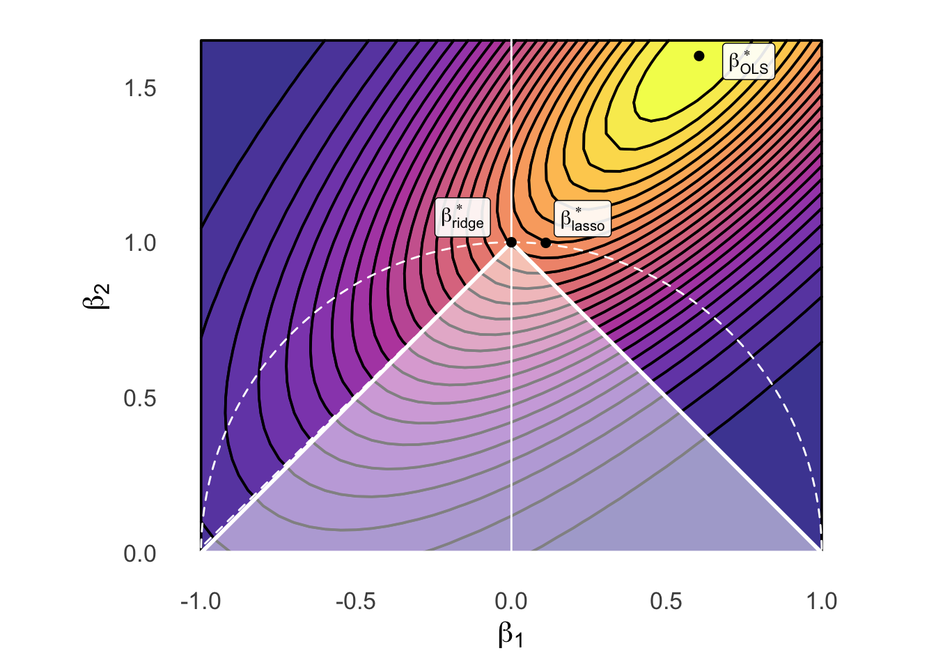

Bayesian Interpretation

Belief \(A\): Most/all of the features you included have important effect on \(Y\)
\(A \implies\) Gaussian prior on \(\beta_j\), \(\mu = 0\)
If \(X \sim \mathcal{N}(\mu, \sigma^2)\), pdf of \(X\) is

\[ f_X(x) = \frac{1}{\sqrt{2\pi \sigma^2}}\exp\left[ -\frac{1}{2}\left( \frac{x-\mu}{\sigma}\right)^2 \right] \]

Code

library(tidyverse) |> suppressPackageStartupMessages()
library(latex2exp) |> suppressPackageStartupMessages()
prior_labs <- labs(
  x = TeX("$\\beta_j$"),
  y = TeX("$f(\\beta_j)$")
)
ggplot() +
  stat_function(fun=dnorm, linewidth=1) +
  xlim(-3, 3) +
  theme_dsan(base_size=28) +
  prior_labs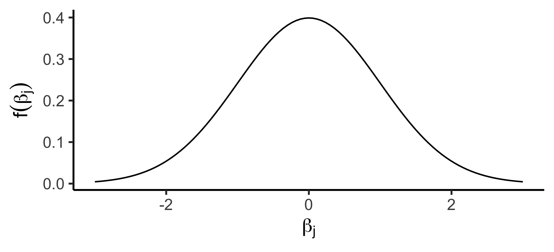

Gaussian prior \(\leadsto\) Ridge Regression!
(High complexity penalty \(\lambda\) \(\leftrightarrow\) low \(\sigma^2\))

Belief \(B\): Only a few of the features you included have important effect on \(Y\)
\(B \implies\) Laplacian prior on \(\beta_j\), \(\mu = 0\)
If \(X \sim \mathcal{L}(\mu, b)\), pdf of \(X\) is

\[ f(x) = \frac{1}{2b}\exp\left[ -\left| \frac{x - \mu}{b} \right| \right] \]

Code

library(tidyverse) |> suppressPackageStartupMessages()
library(latex2exp) |> suppressPackageStartupMessages()
library(extraDistr) |> suppressPackageStartupMessages()
ggplot() +
  stat_function(fun=dlaplace, linewidth=1) +
  xlim(-3, 3) +
  theme_dsan(base_size=28) +
  prior_labs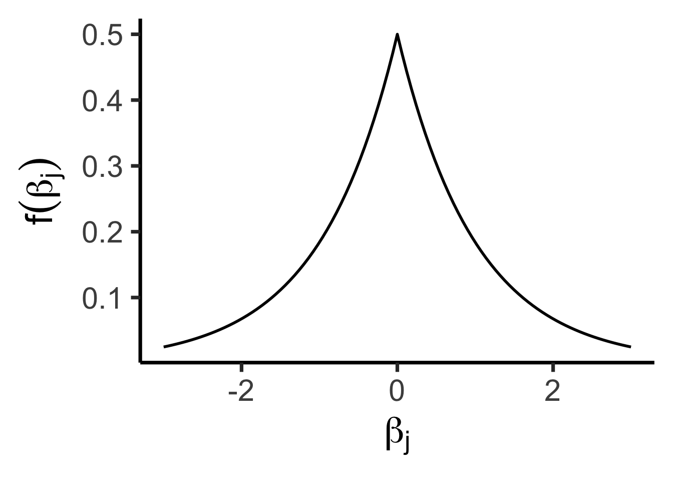

Laplacian prior \(\leadsto\) Lasso!
(High complexity penalty \(\lambda\) \(\leftrightarrow\) low \(b\))

Ok So… How Do We Find These Magical \(\lambda\) Values?

Cross-Validation!
(…that’s, uh, that’s it! That’s the whole slide!)
(But let’s look at what we find when we use CV…)

Varying \(\lambda\) \(\leadsto\) Tradeoff Curve!

Ridge Regression Case:

Increasing \(\lambda\) in \(\displaystyle \min_{\boldsymbol\beta}\left[\text{RSS} + \lambda \| \boldsymbol\beta \|_2^2 \right]\)

\(\equiv\)

Decreasing \(s\) in \(\displaystyle \min_{\boldsymbol\beta}\left[ \text{RSS} \right] \text{ s.t. }\|\boldsymbol\beta\|_2^2 \leq s\)

Only Change: \(L^1\) instead of \(L^2\) Norm 🤯

Lasso Case:

Increasing \(\lambda\) in \(\displaystyle \min_{\boldsymbol\beta}\left[\text{RSS} + \lambda \| \boldsymbol\beta \|_1\right]\)

\(\equiv\)

Decreasing \(s\) in \(\displaystyle \min_{\boldsymbol\beta}\left[ \text{RSS} \right] \text{ s.t. }\|\boldsymbol\beta\|_1 \leq s\)

Week 7 Preview: Linear Functions

You’ve already seen polynomial regression:

\[ Y = \beta_0 + \beta_1X + \beta_2X^2 + \beta_3X^3 + \cdots + \beta_d X^d \]

Plus (technically) “Fourier regression”:

\[ \begin{align*} Y = \beta_0 + \beta_1 \cos(\pi X) + \beta_2 \sin(\pi X) + \cdots + \beta_{2d-1}\cos(\pi d X) + \beta_{2d}\sin(\pi d X) \end{align*} \]

New Regression Just Dropped

Piecewise regression:

Choose \(K\) cutpoints \(c_1, \ldots, c_K\)

Let \(C_k(X) = \mathbb{1}[c_{k-1} \leq X < c_k]\), (\(c_0 \equiv -\infty\), \(c_{K+1} \equiv \infty\))

\[ Y = \beta_0 + \beta_1C_1(X) + \beta_2C_2(X) + \cdots + \beta_KC_K(X) \]

Decomposing Fancy Regressions into Core “Pieces”

Q: What do all these types of regression have in common?
A: They can all be written in the form

\[ Y = \beta_0 + \beta_1 b_1(X) + \beta_2 b_2(X) + \cdots + \beta_d b_d(X) \]
Where \(b(\cdot)\) is called a basis function
- Linear (\(d = 1\)): \(b_1(X) = X\)
- Polynomial: \(b_j(X) = X^j\)
- Piecewise: \(b_j(X) = \mathbb{1}[c_{j-1} \leq X < c_j]\)

	Low Variance	High Variance
Low Bias
High Bias