Week 12: Survival Analysis

DSAN 5300: Statistical Learning
Spring 2025, Georgetown University

Author

Affiliation

Jeff Jacobs

jj1088@georgetown.edu

Open slides in new tab →

Schedule

Today’s Planned Schedule:

	Start	End	Topic
Lecture	6:30pm	7:00pm	Estimating Survival Curves →
	7:00pm	7:20pm	Comparing Between Groups →
	7:20pm	8:00pm	Regression (Cox Proportional Hazard Model) →
Break!	8:00pm	8:10pm
	8:10pm	9:00pm	Quiz 3 →

source("../dsan-globals/_globals.r")
set.seed(5300)

$$$$

Roadmap

• Basic tool: survival curve $S(t)$ = probability of surviving past period $t$
• Complicating factor: Censored obs (e.g., drop out of study)
• $\Rightarrow$ Need to think about DGP: Why is observation $i$ censored while $j$ is observed?
  • Basic estimators only valid if censoring $\perp$ survival time
• How to compare survival between two groups
• Regression: Effect of features $X_1,\dots ,X_p$ on survival

Survival Analysis Basics

• Lots of information crunched into this one figure!

ISLR Figure 11.1

Read Left to Right $\Rightarrow$ Sequence of Events

Modified ISLR Figure 11.1

“Slice” at Deaths $\Rightarrow$ At-Risk Observations

Modified ISLR Figure 11.1

The Actual Dataset We Get

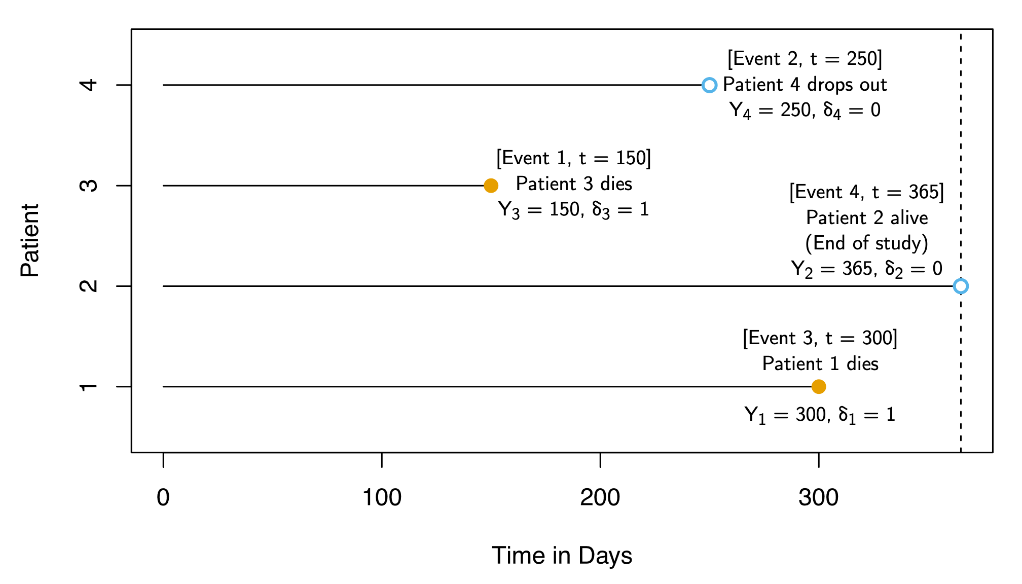
Patient ($i$)	Observed Outcome ($Y_i$)	Observed? (${\delta }_i$)
1	300	1
2	365	0
3	150	1
4	250	0

The Dataset We Can Infer

Patient ($i$)	$Y_i$	${\delta }_i$	Survival Time ($T_i$)	Censor Point ($C_i$)
1	300	1	300	NA
2	365	0	NA	365
3	150	1	150	NA
4	250	0	NA	250

…If we’re testing effect of treatment, which column do we most care about?

Measuring Effect of Treatment!

Patient ($i$)	$Y_i$	${\delta }_i$	Survival Time ($T_i$)	Censor Point ($C_i$)
1	300	1	300	NA
2	365	0	NA	365
3	150	1	150	NA
4	250	0	NA	250

…If we’re testing effect of treatment, $T_i$ is what we care about!

Basic Question 1: Survival

• Let $T$ be a RV representing time of death for a patient
• What is probability that patient survives past given time $t$?

$$S_T(t)=Pr(T>t)$$

• Note relationship to something you saw in 5100!
• $S_T(t)$ defined to be $1-F_T(t)$, where $F_T(t)$ is CDF of $T$:

$$F_T(t)=Pr(T\le t)$$

Kaplan-Meier Estimator: Intuition

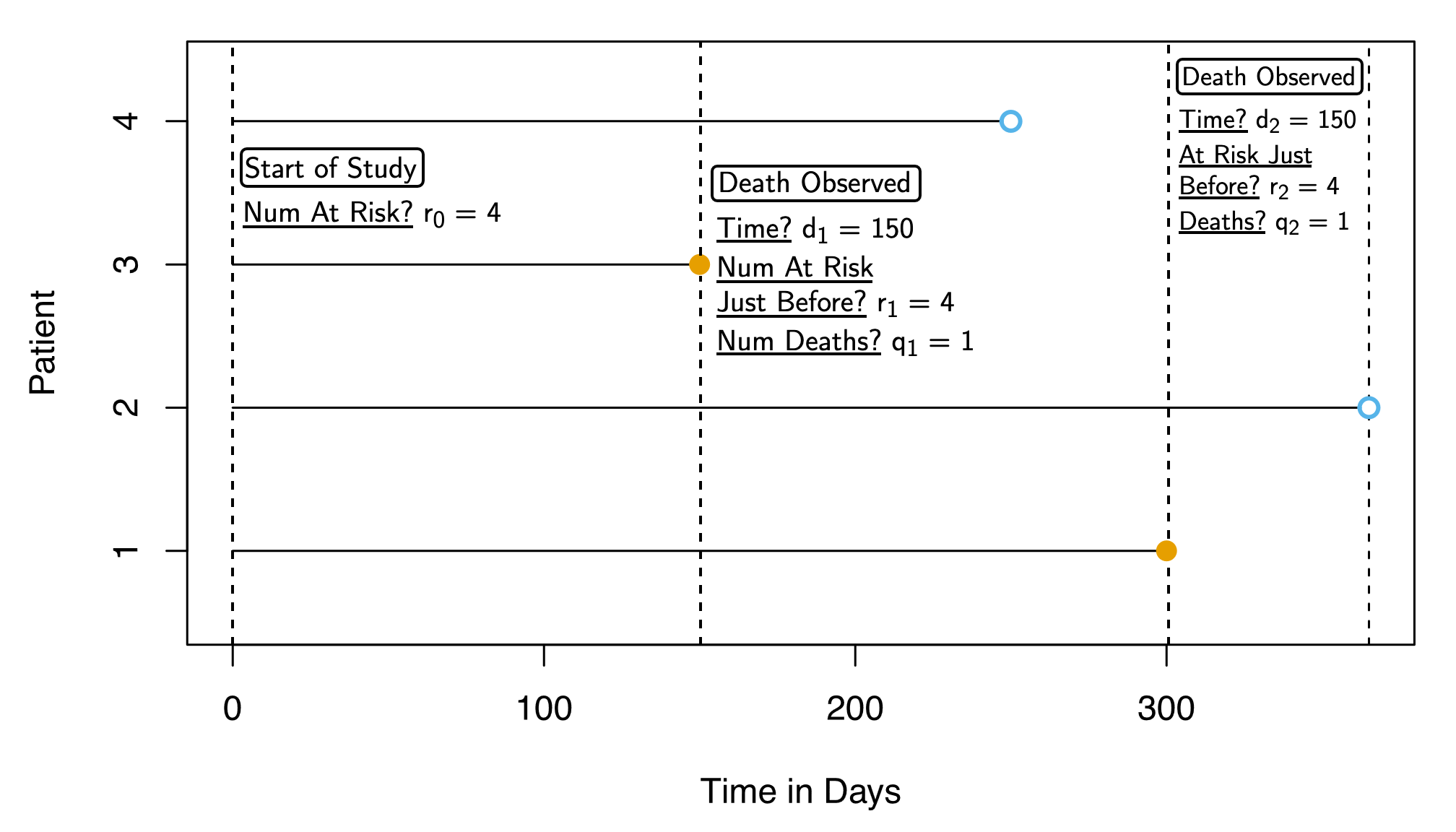
Each death event $d_k$ gives us info that survival probability lower by some amount

Break $S(t)$ into sequence of stepwise changes at $d_1,\dots ,d_K$:

$$\begin{array}{rl}S(d_k)=Pr(T>d_k)& \stackrel{\text{LTP}}{=}Pr(T>d_k\mid T>d_{k-1})\stackrel{S(d_{k-1})}{\overbrace{Pr(T>d_{k-1})}}\\ & \phantom{=}+\underset{\text{Contradiction}⟹Pr=0}{\underbrace{Pr(T>d_k\mid T\le d_{k-1})}}Pr(T\le d_{k-1})\end{array}$$

Gives us a recurrence relation:

$$\begin{array}{rl}S(d_k)& =Pr(T>d_k\mid T>d_{k-1})S(d_{k-1})\\ S(d_{k-1})& =Pr(T>d_{k-1}\mid T>d_{k-2})S(d_{k-2})\\ & ⋮\\ S(d_2)& =Pr(T>d_2\mid T>d_1)S(d_1)\\ S(d_1)& =Pr(T>d_1\mid T>d_0)S(d_0)=Pr(T>d_1)\end{array}$$

Plug each eq into eq above it to derive:

$$\begin{array}{rl}S(d_k)=& Pr(\underset{\text{Survives past }{d}_k}{\underbrace{T>d_k}}\mid \underset{\text{Survives past }{d}_{k-1}}{\underbrace{T>d_{k-1}}})\\ & \times Pr(\underset{\text{Survives past }{d}_{k-1}}{\underbrace{T>d_{k-1}}}\mid \underset{\text{Survives past }{d}_{k-2}}{\underbrace{T>d_{k-2}}})\\ & \times \cdots \times Pr(\underset{\text{Survives past }{d}_2}{\underbrace{T>d_2}}\mid \underset{\text{Survives past }{d}_1}{\underbrace{T>d_1}})\\ & \times Pr(\underset{\text{Survives past }{d}_1}{\underbrace{T>d_1}})\end{array}$$

Kaplan-Meier Estimator

• Defined at death points $d_k$ as

$$\hat{S}(d_k)=\prod _{j=1}^k(\stackrel{\text{Num Survived}}{\overbrace{\frac{r_j-q_j}{\underset{\text{Num At Risk}}{\underbrace{r_j}}}}})$$

• Then, for $t\in (d_k,d_{k+1})$, $\hat{S}(t)=\hat{S}(d_k)$, producing stepwise survival function:

ISLR Figure 11.2

Kaplan-Meier Estimator for our Example

Two death points: $d_1=150,d_2=300$ (plus start point $d_0=0$)

$$\begin{array}{rl}\hat{S}(d_0)& =\prod _{j=0}^0\left(\frac{r_k-q_k}{r_k}\right)=\left(\frac{4-0}{4}\right)=\boxed{{\displaystyle 1}}\\ \hat{S}(d_1)& =\prod _{j=0}^1\left(\frac{r_k-q_k}{r_k}\right)=\boxed{{\displaystyle 1}}\cdot \left(\frac{r_1-q_1}{r_1}\right)\\ & =\boxed{{\displaystyle 1}}\cdot \left(\frac{4-1}{4}\right)=\boxed{{\displaystyle \frac{3}{4}}}\\ \hat{S}(d_2)& =\prod _{j=0}^2\left(\frac{r_k-q_k}{r_k}\right)=\boxed{{\displaystyle 1}}\cdot \boxed{{\displaystyle \frac{3}{4}}}\cdot \left(\frac{r_2-q_2}{r_2}\right)\\ & =\boxed{{\displaystyle 1}}\cdot \boxed{{\displaystyle \frac{3}{4}}}\cdot \left(\frac{2-1}{2}\right)=\frac{3}{4}\cdot \frac{1}{2}=\boxed{{\displaystyle \frac{3}{8}}}\end{array}$$

library(tidyverse) |> suppressPackageStartupMessages()
library(survival) |> suppressPackageStartupMessages()
library(latex2exp) |> suppressPackageStartupMessages()
surv_df <- tribble(
  ~id, ~y, ~delta,
  1, 300, 1,
  2, 365, 0,
  3, 150, 1,
  4, 250, 0
)
surv_obj <- Surv(surv_df$y, event = surv_df$delta)
surv_model <- survfit(surv_obj ~ 1)
# Plot options
par(mar=c(2,4,1.25,1.0)) # bltr
y_label <- TeX("$\\Pr(T > t)$")
plot(
  surv_model,
  ylab=y_label,
  lwd=1,
  main="Survival Curve for 4-Patient Example"
) # conf.int=FALSE
# Add colors
# lines(c(0, 150), c(1.0, 1.0), type='l', col='#E69F00', lwd=2)
rect(xleft = 0, xright = 150, ybottom = 0, ytop = 1.0, col="#E69F0040", lwd=0)
# lines(c(150, 300), c(3/4, 3/4), type='l', col='#56B4E9', lwd=2)
rect(xleft = 150, xright = 300, ybottom = 0, ytop = 1.0, col="#56B4E940", lwd=0)
# lines(c(300, 365), c(3/8, 3/8), type='l', col='#009E73', lwd=2)
rect(xleft = 300, xright = 365, ybottom = 0, ytop = 1.0, col="#009E7340", lwd=0)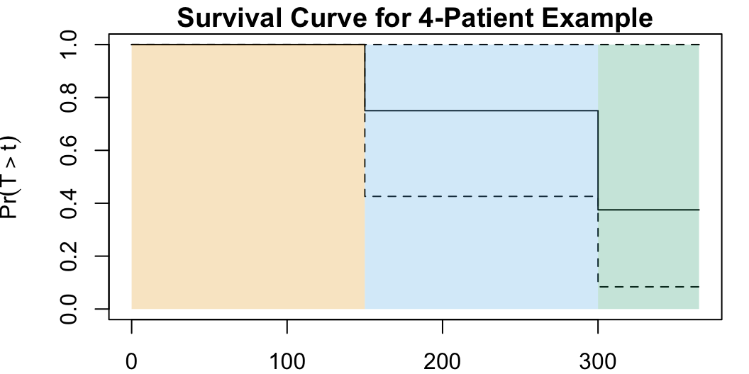

Comparing Survival Curves

• Are female patients more likely to survive than male patients?

ISLR Figure 11.3

Log-Rank Test

• At each death event $d_k$, construct a table like:

	Group 1	Group 2	Total
Died	$q_{1k}$	$q_{2k}$	$q_k$
Survived	$r_{1k}-q_{1k}$	$r_{2k}-q_{2k}$	$r_k-q_k$
Total	$r_{1k}$	$r_{2k}$	$r_k$

• Focus on $q_{1k}$! Null hypothesis: across all $k\in \{1,\dots ,K\}$, $q_{1k}$ not systematically lower or higher than RHS:

$$\mathbb{E}[\underset{\begin{array}{c}\text{Group 1 deaths}\\ \text{at }{d}_k\end{array}}{\underbrace{q_{1k}}}]=\stackrel{\begin{array}{c}\text{At risk in}\\ \text{Group 1}\end{array}}{\overbrace{r_{1k}}}\cdot \underset{\text{Overall death rate at }{d}_k}{\underbrace{\left(\frac{q_k}{r_k}\right)}}$$

Log-Rank Test Statistic

• Test statistic $W$ should “detect” the alternative hypothesis, on basis of information $X$… We can use $\boxed{{\displaystyle X=\sum _{k=1}^K{q}_{1k}}}$!
• Here, log-rank test statistic $W$ detects how much $q_{1k}$ deviates from expected value from prev slide:

$$\begin{array}{rl}W& =\frac{X-\mathbb{E}[X]}{\sqrt{\text{Var}[X]}}=\frac{\sum _{k=1}^K{q}_{1k}-\mathbb{E}\left[\sum _{k=1}^K{q}_{1k}\right]}{\sqrt{\text{Var}\left[\sum _{k=1}^K{q}_{1k}\right]}}=\frac{\sum _{k=1}^K(q_{1k}-\mathbb{E}[q_{1k}])}{\sqrt{\text{Var}\left[\sum _{k=1}^K{q}_{1k}\right]}}\\ & =\frac{\sum _{k=1}^K(q_{1k}-r_{1k}\cdot \frac{q_k}{r_k})}{\sqrt{\text{Var}\left[\sum _{k=1}^K{q}_{1k}\right]}}\underset{\text{Ex 11.7}}{\stackrel{\text{ISLR}}{=}}\frac{\sum _{k=1}^K(q_{1k}-r_{1k}\cdot \frac{q_k}{r_k})}{\sqrt{\sum _{k=1}^K\frac{q_k(r_{1k}/r_k)(1-r_{1k}/r_k)(r_k-q_k)}{r_k-1}}}\end{array}$$

Regression with Survival Response

The Hazard Function

• Death rate at tiny instant after $t$ (between $t$ and $t+\mathrm{\Delta }t$), given survival past $t$:

$$h(t)\stackrel{\text{def}}{=}\underset{\mathrm{\Delta }t\to 0}{lim}\frac{Pr(t<T\le t+\mathrm{\Delta }t)}{\mathrm{\Delta }t}$$

• If we define a RV $T_{>t}\stackrel{\text{def}}{=}[T\mid T>t]$, $h(t)$ is the pdf of $T_{>t}$!
• Can relate $h(t)$ to quantities we know (e.g., from 5100):

$$\underset{\text{pdf of }{T}_{>t}}{\underbrace{h(t)}}=\frac{\stackrel{\text{pdf of }T}{\overbrace{f(t)}}}{\underset{Pr(T>t)}{\underbrace{S(t)}}}$$

Proportional Hazard Assumption

$$h(t\mid x_i)=h_0(t)\exp \left[\sum _{j=1}^p{\beta }_j{x}_{ij}\right]⟺\underset{\hslash (t\mid x_i)}{\underbrace{\log [h(t\mid x_i)]}}=\underset{{\hslash }_0(t)}{\underbrace{\log [h_0(t)]}}+\sum _{j=1}^p{\beta }_j{x}_{ij}$$

Basically: Features $X_j$ shift [log] baseline hazard function ${\hslash }_0(t)$ up and down by constant amounts, via multiplication by $e^{{\beta }_j}$

• Top row: ${\hslash }_0(t)$ in black, $X_j=1$ shifts it down via multiplication by $e^{{\beta }_j}$ to form $\hslash (t\mid X_j)$ in green
• Bottom row: Proportional hazard violated, since $X_j=1$ associated with different changes to ${\hslash }_0(t)$ at different $t$ values

Cox Proportional Hazard Model

• Intuition: Best $\beta$s are those which best predict $i$’s death among all at risk at same time. Called “Partial Likelihood” $\text{PL}(\mathit{\beta })$ since we don’t need to estimate $h_0(t)$!

$$\prod _{i:{\delta }_i=1}\frac{\cancel{h_0(t)}\exp \left[\sum _{j=1}^p{\beta }_j{x}_{ij}\right]}{{\displaystyle \sum _{i^{\prime }:y_{i^{\prime }}\ge y_i}}\cancel{h_0(t)}\exp \left[\sum _{j=1}^p{\beta }_j{x}_{i^{\prime }j}\right]}=\prod _{i:{\delta }_i=1}\frac{\exp \left[\sum _{j=1}^p{\beta }_j{x}_{ij}\right]}{{\displaystyle \sum _{i^{\prime }:y_{i^{\prime }}\ge y_i}}\exp \left[\sum _{j=1}^p{\beta }_j{x}_{i^{\prime }j}\right]}$$

• Also note the missing intercept ${\beta }_0$: handled by the baseline hazard function $h_0(t)$ (which we cancel out anyways!)

In Code

• We’ll use the survival library in R, very similar syntax to lm(), glm(), etc.!

library(survival) |> suppressPackageStartupMessages()
library(ISLR2) |> suppressPackageStartupMessages()
bc_df <- BrainCancer |> filter(diagnosis != "Other")
bc_df$diagnosis = factor(bc_df$diagnosis)
bc_df$sex <- factor(substr(bc_df$sex, 1, 1))
bc_df$loc <- factor(substr(bc_df$loc, 1, 5))
options(width=130)
summary(bc_df)

 sex         diagnosis     loc           ki              gtv         stereo       status           time      
 F:39   Meningioma:42   Infra:10   Min.   : 40.00   Min.   : 0.040   SRS:19   Min.   :0.000   Min.   : 0.07  
 M:34   LG glioma : 9   Supra:63   1st Qu.: 80.00   1st Qu.: 2.500   SRT:54   1st Qu.:0.000   1st Qu.: 9.77  
        HG glioma :22              Median : 80.00   Median : 6.480            Median :0.000   Median :26.46  
                                   Mean   : 81.37   Mean   : 8.297            Mean   :0.411   Mean   :27.83  
                                   3rd Qu.: 90.00   3rd Qu.:11.380            3rd Qu.:1.000   3rd Qu.:41.44  
                                   Max.   :100.00   Max.   :33.690            Max.   :1.000   Max.   :82.56  

bc_df |> head(5)

sex	diagnosis	loc	ki	gtv	stereo	status	time
F	Meningioma	Infra	90	6.11	SRS	0	57.64
M	HG glioma	Supra	90	19.35	SRT	1	8.98
F	Meningioma	Infra	70	7.95	SRS	0	26.46
F	LG glioma	Supra	80	7.61	SRT	1	47.80
M	HG glioma	Supra	90	5.06	SRT	1	6.30

coxph() Estimation

library(broom) |> suppressPackageStartupMessages()
full_cox_model <- coxph(
  Surv(time, status) ~ sex + diagnosis + loc + ki + gtv + stereo,
  data=bc_df
)
broom::tidy(full_cox_model) |> mutate_if(is.numeric, round, 3)

term	estimate	std.error	statistic	p.value
sexM	0.456	0.396	1.154	0.249
diagnosisLG glioma	0.864	0.641	1.347	0.178
diagnosisHG glioma	2.116	0.470	4.504	0.000
locSupra	1.482	1.105	1.342	0.180
ki	-0.048	0.020	-2.406	0.016
gtv	0.036	0.026	1.361	0.173
stereoSRT	-0.475	0.591	-0.803	0.422

• Diagnosis: Relative to baseline of Meningioma, HG (High-Grade) glioma associated with $e^{2.155}\approx 8.628$ times greater hazard
• Karnofsky Index (ki): 1-unit increase associated with reduction of hazard to $e^{-0.055}\approx 94.65$% of previous value [0-100 scale of self-functioning abilities]

Survival Curves for Each Diagnosis

library(extrafont) |> suppressPackageStartupMessages()
par(cex=1.2, family="CMU Sans Serif")
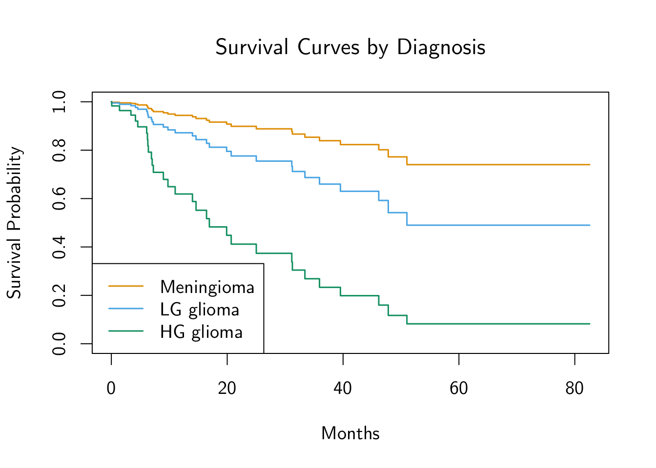
diag_levels <- c("Meningioma", "LG glioma", "HG glioma")
diag_df <- tibble(
  diagnosis = diag_levels,
  sex = rep("F", 3),
  loc = rep("Supra", 3),
  ki = rep(mean(bc_df$ki), 3),
  gtv = rep(mean(bc_df$gtv), 3),
  stereo = rep("SRT", 3)
)
survplots <- survfit(full_cox_model, newdata = diag_df)
plot(
  survplots,
  main = "Survival Curves by Diagnosis",
  xlab = "Months", ylab = "Survival Probability",
  col = cb_palette, lwd=1.5
)
legend(
  "bottomleft",
  diag_levels,
  col = cb_palette, lty = 1, lwd=1.5
)

Less Straightforward: Curves for Each ki, gtv Val

• Technically a different survival curve for each value of ki $\in [0,100]$, gtv $\in (0,\mathrm{\infty })$

bc_df |> ggplot(aes(x=ki)) +
  geom_density(
    linewidth=g_linewidth,
    fill=cb_palette[1], alpha=0.333
  ) +
  theme_dsan(base_size=28) +
  labs(title = "Karnofsky Index Distribution")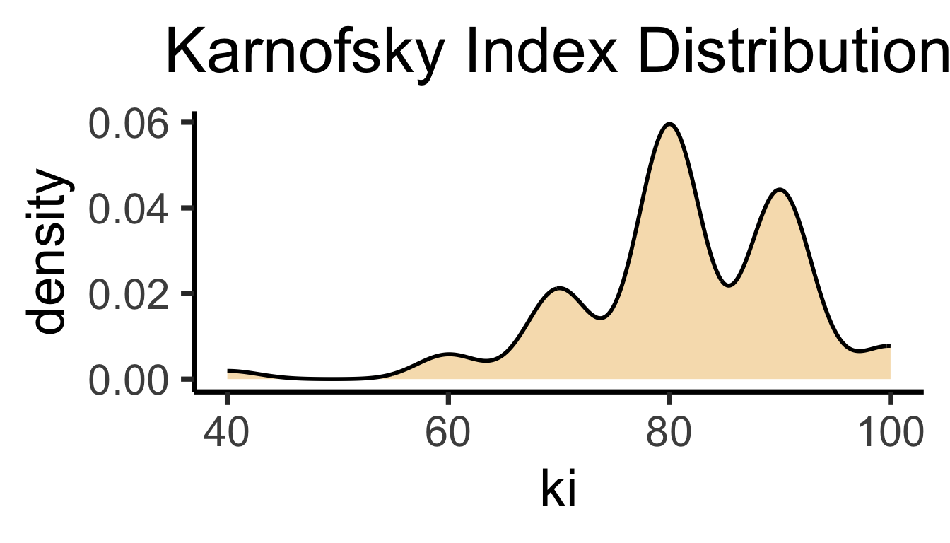

bc_df |> ggplot(aes(x=gtv)) +
  geom_density(
    linewidth=g_linewidth,
    fill=cb_palette[1], alpha=0.333
  ) +
  theme_dsan(base_size=28) +
  labs(title = "Gross Tumor Volume (GTV) Distribution")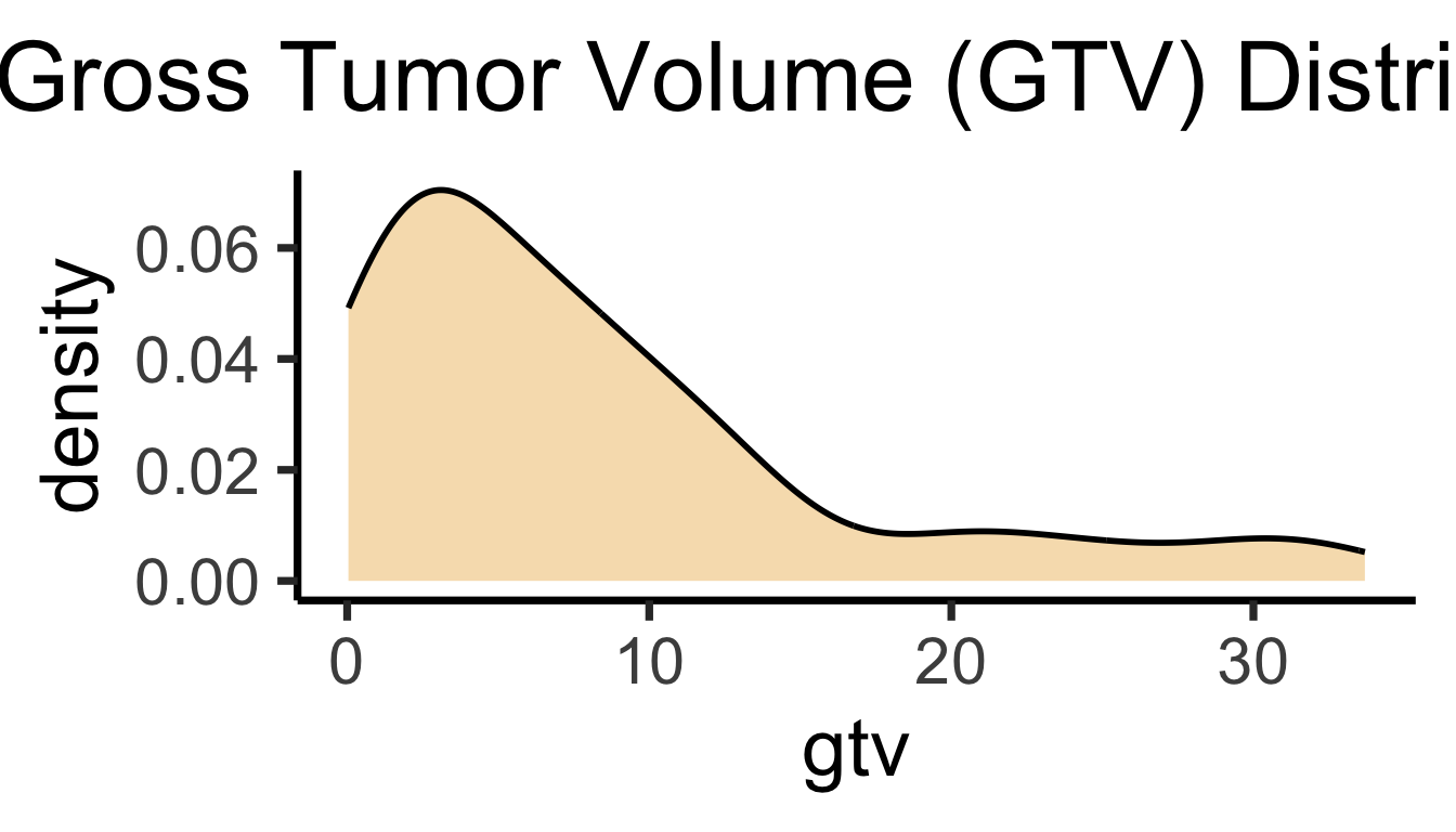

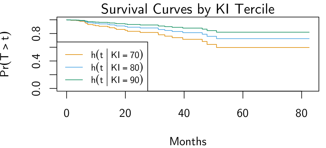
• One approach: bin into (low, medium, high) via terciles, one curve per bin median:

ki_terciles <- quantile(bc_df$ki, c(1/3, 2/3))
bc_df <- bc_df |> mutate(
  tercile = ifelse(ki < ki_terciles[1], 1, ifelse(ki < ki_terciles[2], 2, 3))
)
(terc_df <- bc_df |>
  group_by(tercile) |>
  summarize(med_ki=median(ki)))

tercile	med_ki
1	70
2	80
3	90

library(latex2exp) |> suppressPackageStartupMessages()
ki_df <- tibble(
  diagnosis = rep("Meningioma", 3),
  sex = rep("F", 3),
  loc = rep("Supra", 3),
  ki = terc_df$med_ki,
  gtv = rep(mean(bc_df$gtv), 3),
  stereo = rep("SRT", 3)
)
ki_plots <- survfit(full_cox_model, newdata = ki_df)
par(
  mar=c(4.0,4.0,1.2,0.5),
  cex=1.2,
  family="CMU Sans Serif"
) # bltr
plot(
  ki_plots,
  main = "Survival Curves by KI Tercile",
  xlab = "Months",
  ylab = TeX("$\\Pr(T > t)$"),
  lwd = 1,
  col = cb_palette
)
ki_labs <- c(
  TeX("$h( t \\, | \\, KI = 70 )$"),
  TeX("$h( t \\, | \\, KI = 80 )$"),
  TeX("$h( t \\, | \\, KI = 90 )$")
)
legend(
  "bottomleft",
  ki_labs, lwd=1,
  col = cb_palette, lty = 1, cex=0.8
)

Quiz 3

• Last one! You got this, حَبَائب!