Week 5: Cross-Validation for Model Assessment

DSAN 5300: Statistical Learning
Spring 2025, Georgetown University

Author

Affiliation

Jeff Jacobs

jj1088@georgetown.edu

Open slides in new tab →

Schedule

Today’s Planned Schedule:

	Start	End	Topic
Lecture	6:30pm	6:50pm	Roadmap: Week 4 $⇝$ Week 6 →
	6:50pm	7:20pm	Non-Linear Data-Generating Processes →
	7:20pm	8:00pm	Validation: Evaluating Non-Linear Models →
Break!	8:00pm	8:10pm
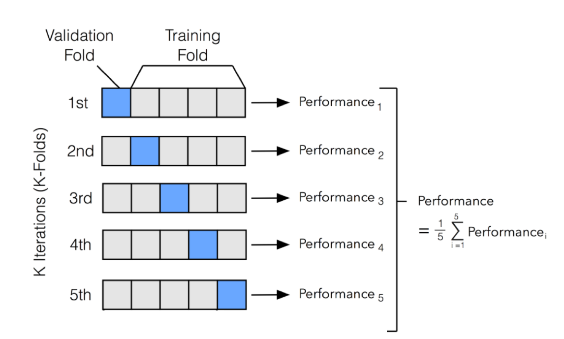
	8:10pm	9:00pm	$K$-Fold Cross-Validation: Cooking with Gas →

source("../dsan-globals/_globals.r")
set.seed(5300)

$$$$

Roadmap

• [Week 4] Oh no! When we go beyond linear models, we have to worry about overfitting!
  • $⟹$ New goal! Maximize generalizability rather than accuracy
  • $⟹$ Evaluate models on unseen test data rather than training data
• [Week 5] Cross-Validation (CV) as a tool for Model Assessment: For more complex, non-linear models, is there some way we can try to… “foresee” how well a trained model will generalize?
  • Answer: Yes! Cross-validation!
• [Week 6] Regularization as a tool for Model Selection: Now that we have a method (CV) for imperfectly measuring “generalizability”, is there some way we can try to… allow models to optimize CV but penalize them for unnecessary complexity?
  • Answer: Yes! Regularization methods like LASSO and Elastic Net!

[Reminder (W04)] New Goal: Generalizability

The Goal of Statistical Learning

Find…

• A function $\hat{y}=f(x)$ ✅
• That best predicts $Y$ for given values of $X$ ✅
• For data that has not yet been observed! 😳❓

A Non-Linear Data-Generating Process (DGP)

Our Working DGP

• Each country $i$ has a certain $x_i={\mathtt{\text{gdp\_per\_capita}}}_i$
• They spend some portion of it on healthcare each year, which translates (based on the country’s healthcare system) into health outcomes $y_i$
• We operationalize these health outcomes as $y_i={\mathtt{\text{DALY}}}_i$: Disability Adjusted Life Years, cross-nationally-standardized “lost years of minimally-healthy life”

library(tidyverse) |> suppressPackageStartupMessages()
library(plotly) |> suppressPackageStartupMessages()
daly_df <- read_csv("assets/dalys_cleaned.csv")

Rows: 162 Columns: 6
── Column specification ────────────────────────────────────────────────────────
Delimiter: ","
chr (2): name, gdp_cap
dbl (4): dalys_pc, population, gdp_pc_clean, log_dalys_pc

ℹ Use `spec()` to retrieve the full column specification for this data.
ℹ Specify the column types or set `show_col_types = FALSE` to quiet this message.

daly_df <- daly_df |> mutate(
  gdp_pc_1k=gdp_pc_clean/1000
)
model_labels <- labs(
  x="GDP per capita ($1K PPP, 2021)",
  y="Log(DALYs/n)",
  title="Decrease in DALYs as GDP/n Increases"
)
daly_plot <- daly_df |> ggplot(aes(x=gdp_pc_1k, y=log_dalys_pc, label=name)) +
  geom_point() +
  # geom_smooth(method="loess", formula=y ~ x) +
  geom_smooth(method="lm", formula=y ~ poly(x,5), se=FALSE) +
  theme_dsan(base_size=14) +
  model_labels
ggplotly(daly_plot)

Warning: The following aesthetics were dropped during statistical transformation: label.
ℹ This can happen when ggplot fails to infer the correct grouping structure in
  the data.
ℹ Did you forget to specify a `group` aesthetic or to convert a numerical
  variable into a factor?

$$\begin{array}{rl}⇝Y=& 10.58-0.2346X+0.01396X^2\\ & -0.0004X^3+0.000005X^4\\ & -0.00000002X^5+\epsilon \end{array}$$

eval_fitted_poly <- function(x) {
  coefs <- c(
    10.58,  -0.2346, 0.01396,
    -0.0004156, 0.0000053527, -0.0000000244
  )
  x_terms <- c(x^0, x^1, x^2, x^3, x^4, x^5)
  dot_prod <- sum(coefs * x_terms)
  return(dot_prod)
}
N <- 500
x_vals <- runif(N, min=0, max=90)
y_vals <- sapply(X=x_vals, FUN=eval_fitted_poly)
sim_df <- tibble(gdpc=x_vals, ldalys=y_vals)
ggplot() +
  geom_line(data=sim_df, aes(x=gdpc, y=ldalys)) +
  geom_point(data=daly_df, aes(x=gdp_pc_1k, y=log_dalys_pc)) +
  theme_dsan() +
  model_labels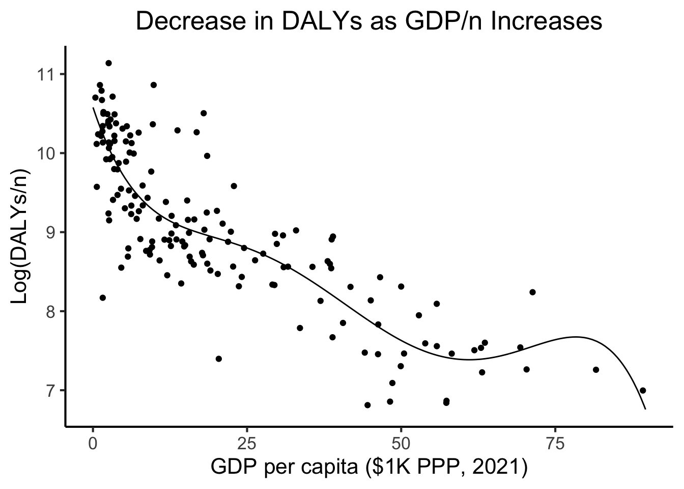

The “True” Model

• From here onwards, we adopt this as our “true” model, for pedagogical purposes!
• Meaning: we use this model to get a sense for how…
  • CV can “foresee” test error $⇝$ confidence in CV
  • Regularization can penalize overly-complex models $⇝$ confidence in LASSO
• In the real world we don’t know the DGP!
  • $⟹$ We build our confidence here, then take off the training wheels irl: use CV/Regularization in hopes they can help us “uncover” the unknown DGP

run_dgp <- function(world_label="Sim", N=60, x_max=90) {
  x_vals <- runif(N, min=0, max=x_max)
  y_raw <- sapply(X=x_vals, FUN=eval_fitted_poly)
  y_noise <- rnorm(N, mean=0, sd=0.8)
  y_vals <- y_raw + y_noise
  sim_df <- tibble(
    gdpc=x_vals,
    ldalys=y_vals,
    world=world_label
  )
  return(sim_df)
}
df1 <- run_dgp("World 1")
df2 <- run_dgp("World 2")
df3 <- run_dgp("World 3")
dgp_df <- bind_rows(df1, df2, df3)
dgp_df |> ggplot(aes(x=gdpc, y=ldalys)) +
  geom_point(aes(color=world)) +
  facet_wrap(vars(world)) +
  theme_dsan(base_size=22) +
  remove_legend() +
  model_labels +
  labs(title="Three Possible Realizations of our DGP")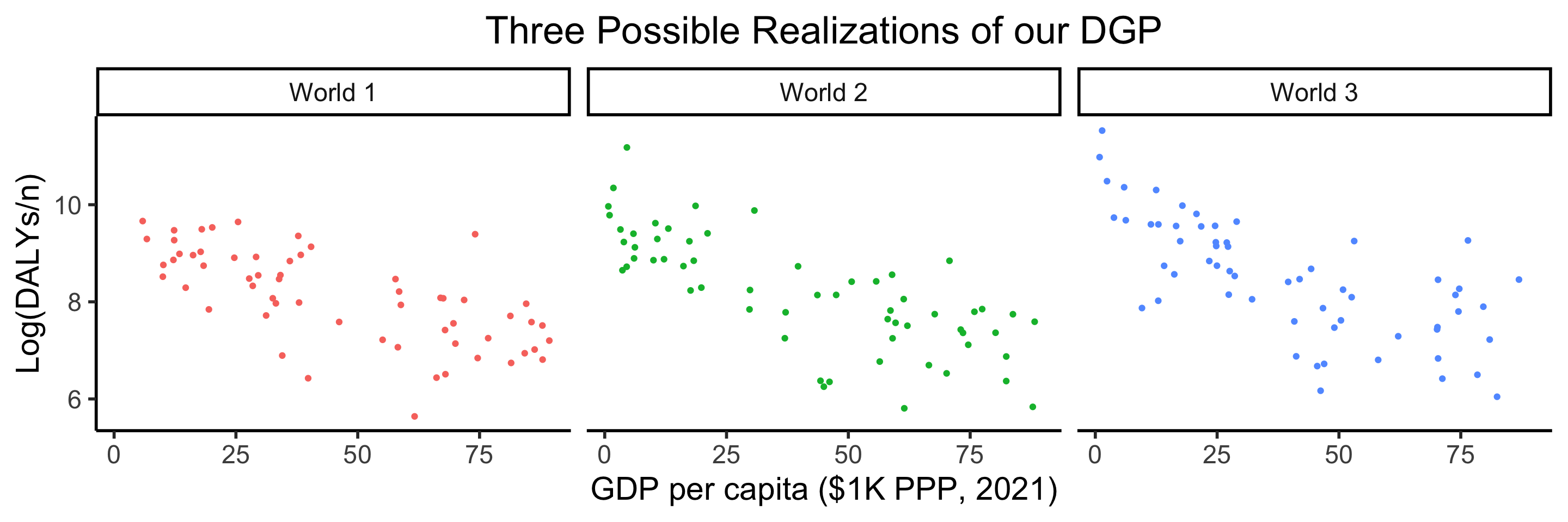

Cross-Validation: Evaluating Non-Linear Models

Specifically: evaluating non-linear models on how well they generalize!

• Beyond the Train-Test Split
• Validation Set
• LOOCV
• $K$-Fold CV

Training vs. Test Data

• We introduced this as a first step towards tackling the scourge of overfitting!

• Training Set $⇝$ Training Error, Test Set $⇝$ Test Error
• So… what’s the issue? Why do we need to complicate this picture?

The Chilling Truth Behind Test Data 🫣

• Science-wise, technically, once you use the test set, you should stop working
• Full gory details in fancy books (Hume (1760) $\to$ Popper (1934)), but the essence is captured by visualizing scientific inference (and statistical learning!) like:

• So, what do we do? Use ${\mathbf{D}}_{\text{Tr}}$ along with knowledge of issues like overfitting to estimate test error!
• Fulfills our goal: find model which best predicts $Y$ from $X$ for unobserved data

The Validation Set Approach

• ⚠️ Remember: under our new goal, “good” models = models that generalize well!
• Optimizing over test set violates scientific inference axioms
• Instead, optimize over training data by “holding out” some portion of it… Enter the Validation Set:

graph grid
{
    graph [
        overlap=true,
        scale=0.2
    ]
    nodesep=0.0
    ranksep=0.0
    rankdir="LR"
    scale=0.2
    node [
        style="filled",
        color=black,
        fillcolor=lightblue,
        shape=box
    ]

    // uncomment to hide the grid
    edge [style=invis]
    
    subgraph cluster_01 {
        label="Training Set (80%)"
        subgraph cluster_02 {
            label="Training Fold (80%)"
            A1[label="16%"] A2[label="16%"] A3[label="16%"] A4[label="16%"]
        }
        subgraph cluster_03 {
            label="Validation Fold (20%)"
            B1[label="16%",fillcolor=lightgreen]
        }
    }
    subgraph cluster_04 {
        label="Test Set (20%)"
    C1[label="20%",fillcolor=orange]
    }
    A1 -- A2 -- A3 -- A4 -- B1 -- C1;
}

Evaluating One Model: Validation Set Approach

• Randomly pick 20% of ${\mathbf{D}}_{\text{train}}$ as sub-training set ${\mathbf{D}}_{\text{SubTr}}$
• The other 80% becomes validation set ${\mathbf{D}}_{\text{Val}}$
• Train model on ${\mathbf{D}}_{\text{SubTr}}$, then evaluate using ${\mathbf{D}}_{\text{Val}}$, to produce validation error $\boxed{{\displaystyle {\epsilon }_{\text{Val}}={\widehat{\text{Err}}}_{\text{Test}}}}$
• ${\epsilon }_{\text{Val}}$ gives us an estimate of the test error
  • $⟹$ this is what we want to optimize, in place of training error, for our new goal 😎!

How Does It Do for Our DGP?

• Recall that the “true” degree is 5, but that you’re not supposed to know that!

library(boot)
set.seed(5300)
sim200_df <- run_dgp(
  world_label="N=200", N=200, x_max=100
)
sim1k_df <- run_dgp(
  world_label="N=1000", N=1000, x_max=100
)
compute_deltas <- function(df, min_deg=1, max_deg=12) {
  cv_deltas <- c()
  for (i in min_deg:max_deg) {
    cur_poly <- glm(ldalys ~ poly(gdpc, i), data=df)
    cur_poly_cv_result <- cv.glm(data=df, glmfit=cur_poly, K=5)
    cur_cv_adj <- cur_poly_cv_result$delta[1]
    cv_deltas <- c(cv_deltas, cur_cv_adj)
  }
  return(cv_deltas)
}
sim200_deltas <- compute_deltas(sim200_df)
sim200_delta_df <- tibble(degree=1:12, delta=sim200_deltas)
sim200_delta_df |> ggplot(aes(x=degree, y=delta)) +
  geom_line() +
  geom_point() +
  geom_vline(xintercept=5, linetype="dashed") +
  scale_x_continuous(
    breaks=seq(from=1,to=12,by=1)
  ) +
  theme_dsan(base_size=22) +
  labs(title="N = 200")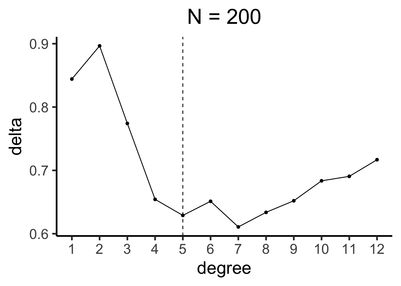

Here, validation error fails to capture ‘true’ model (likely culprits: low $N$, high noise…)

• Possible resolution: [See coming slides!]

sim1k_deltas <- compute_deltas(sim1k_df)
sim1k_delta_df <- tibble(degree=1:12, delta=sim1k_deltas)
sim1k_delta_df |> ggplot(aes(x=degree, y=delta)) +
  geom_line() +
  geom_point() +
  geom_vline(xintercept=5, linetype="dashed") +
  scale_x_continuous(
    breaks=seq(from=1,to=12,by=1)
  ) +
  theme_dsan(base_size=22) +
  labs(title="N = 1000")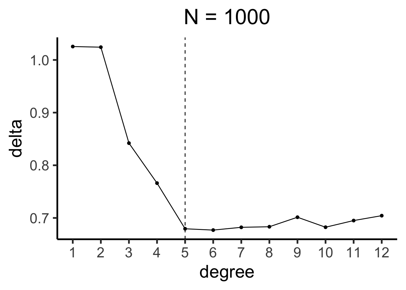

Here, validation error fails to sharply distinguish $d\in \{5,6,7,8\}$

• Possible resolution: “one standard error rule”

Optimizing over Many Models

• Let $\mathfrak{M}=({\mathcal{M}}_1,\dots ,{\mathcal{M}}_D)$ be a set of $D$ different models
  • Ex: ${\mathcal{M}}_1$ could be a linear model, ${\mathcal{M}}_2$ a quadratic model, ${\mathcal{M}}_3$ a cubic model, and so on…
• For each ${\mathcal{M}}_i\in \mathfrak{M}$ (and for given training data ${\mathbf{D}}_{\text{Tr}}$):
  • Use [Insert Validation Approach] to derive ${\epsilon }_i$
• Model ${\mathcal{M}}_i$ with lowest ${\epsilon }_i$ wins!
• We are now cooking with gas! We can use CV to optimize over e.g. HYPERPARAMETERS 🤯 (that we had to just kind of… guess before)!

Cooking with Even More Gas!

(加 even more 油!)

• It turns out that, for the purposes of estimating test error (aka, estimating how well the fitted model will generalize), Validation Set Approach is the worst approach (still good, just, least good!)
• To see its limitations, consider: is there something special about the 20% of data we selected for the validation set?
• Answer: No! It was literally randomly selected!
• $⟹$ Any other 20% “chunk” (which we’ll call a fold from now on) could work just as well

5-Fold Cross-Validation

• Secretly, by choosing a 20% fold to be the validation set earlier, I was priming you for 5-fold cross-validation!

Image Source

$K$-Fold Cross-Validation

• 5 was an arbitrary choice!
  • (Though, one with important and desirable statistical properties, which we’ll get to ASAP)
• In general, $K$-Fold CV Estimator ${\epsilon }_{(K)}={\widehat{\text{Err}}}_{\text{Test}}$ given by

$${\epsilon }_{(K)}=\frac{1}{K}\sum _{i=1}^K{\epsilon }_i^{\text{Val}}$$

Leave-One-Out Cross-Validation (LOOCV)

• $K$-Fold CV with $K:=N$
• Produces the maximum possible number of terms in the summation that leads to ${\epsilon }_{(K)}$
  • i.e., ${\epsilon }_{(N)}$ is an average over the maximum possible number of models
• So… does this mean it’s the best choice?
• Hint: How “different” are any two models used in the sum?

$$\begin{array}{rl}{\epsilon }_{(N)}=& \text{Err}({\mathbf{D}}_1\mid {\mathbf{D}}_{2:100})+\text{Err}({\mathbf{D}}_2\mid {\mathbf{D}}_1,{\mathbf{D}}_{3:100})\\ & +\text{Err}({\mathbf{D}}_3\mid {\mathbf{D}}_{1:2},{\mathbf{D}}_{4:100})+\cdots +\text{Err}({\mathbf{D}}_{100}\mid {\mathbf{D}}_{1:99})\end{array}$$

• The terms here are highly correlated!
• Fun math results around how $K=5$ or $K=10$ can best strike a balance between overly-correlated terms ($K=N$) and not averaging enough models ($K=2$)!

References

Hume, David. 1760. An Enquiry Concerning Human Understanding. Simon and Schuster.

Popper, Karl R. 1934. The Logic of Scientific Discovery. Psychology Press.