Week 13: Machine Learning for Causal Inference

DSAN 5300: Statistical Learning
Spring 2025, Georgetown University

Class Sessions

Author

Affiliation

Jeff Jacobs

jj1088@georgetown.edu

Published

Monday, April 14, 2025

Open slides in new tab →

Schedule

Today’s Planned Schedule:

	Start	End	Topic
Lecture	6:30pm	7:00pm	Fundamental Problem of Causal Inference →
	7:00pm	7:20pm	Apples to Apples →
	7:20pm	8:00pm	How Can Machine Learning Help? →
Break!	8:00pm	8:10pm
	8:10pm	9:00pm	Causal Forests →

Roadmap

What makes causation different from correlation?

Why can’t we use, e.g., Regression to infer causal effects? \(\uparrow X\) by 1 unit ~~causes~~ \(\uparrow Y\) by \(\beta\) units?
\(\leadsto\) Fundamental Problem of Causal Inference

Key to resolving Fundamental Problem: Match similar observations

Apples to apples: If \(j\) receives drug while \(i\) doesn’t, and they’re \(s_{ij}\%\) similar otherwise (age, height)…
Higher \(s_{ij}\) \(\implies\) more confidence in attributing difference in outcomes \(\boxed{\Delta y = y_j - y_i}\) to drug!
\(\leadsto\) Propensity Score Matching (\(\approx\) Logistic Regression)

How can ML help us infer counterfactual effects?

Patient \(i\) didn’t receive treatment, reported VAS pain level \(y^0_i = 80\)…
If \(i\) had received treatment, what would their pain level \(y_i^1\) be?
\(\leadsto\) Causal Forests, to estimate \(\boxed{\Delta y_i = y^1_i - y^0_i}\)

The Fundamental Problem of Causal Inference

The only workable definition of “\(X\) causes \(Y\)”:

Defining Causality (Hume 1739)

\(X\) causes \(Y\) if and only if:

\(X\) temporally precedes \(Y\) and
- In two worlds \(W_0\) and \(W_1\) where everything is exactly the same…
- …except that \(\boxed{X = 0 \text{ in } W_0}\) and \(\boxed{X = 1 \text{ in } W_1}\),
- \(\boxed{Y = 0 \text{ in } W_0}\) and \(\boxed{Y = 1 \text{ in } W_1}\).

The problem? We live in one world, not two simultaneous worlds 😭

Can’t We Just Use Temporal Precedence?

Can’t we just pretend that \(W_0\) is our world at time \(t\) and \(W_1\) is our world at time \(t + 1\)?
Did throwing the eraser at Sam at time \(t\) cause him to be upset at time \(t + 1\)?
No, because at time \(t\), simultaneous with my eraser-throwing, a cockroach scuttled across his foot, the true cause of him being upset at time \(t + 1\)
Without knowing that the worlds are identical except for the posited cause-event, we can’t exclude the possibility of some other cause-event

Extreme Example: Super Mario 64 Speedrunning

Seemingly-reasonable assumption: Button-pushes cause outcomes in games…

During the race, an ionizing particle from outer space collided with DOTA_Teabag’s N64, flipping the eighth bit of Mario’s first height byte. Specifically, it flipped the byte from 11000101 to 11000100, from “C5” to “C4”. This resulted in a height change from C5837800 to C4837800, which by complete chance, happened to be the exact amount needed to warp Mario up to the higher floor at that exact moment.

This was tested by pannenkoek12 - the same person who put up the bounty - using a script that manually flipped that particular bit at the right time, confirming the suspicion of a bit flip.

What About A-B Testing?

Gets us significantly closer, but methods for recovering causal effect require a condition called SUTVA
Stable Unit Treatment Value Assumption: Treatment applied to \(i\) does not affect outcome for another person \(j\)
If we A-B test an app redesign (A = old design, B = new design), and outcome = length of time spent on app…
Person \(i\) seeing design A may like the new design, causing them to spend more time on the app
Person \(i\) may then message person \(j\) “Check out [app], they redesigned everything!”, causing \(j\) to spend more time on app regardless of treatment (network spillover ❌)

What Is To Be Done?

Matching Estimators

Case Study: Military Inequality \(\leadsto\) Military Success

Lyall (2020): “Treating certain ethnic groups as second-class citizens […] leads victimized soldiers to subvert military authorities once war begins. The higher an army’s inequality, the greater its rates of desertion, side-switching, and casualties”

Matching constructs pairs of belligerents that are similar across a wide range of traits thought to dictate battlefield performance but that vary in levels of prewar inequality. The more similar the belligerents, the better our estimate of inequality’s effects, as all other traits are shared and thus cannot explain observed differences in performance, helping assess how battlefield performance would have improved (declined) if the belligerent had a lower (higher) level of prewar inequality.

Since [non-matched] cases are dropped […] selected cases are more representative of average belligerents/wars than outliers with few or no matches, [providing] surer ground for testing generalizability of the book’s claims than focusing solely on canonical but unrepresentative usual suspects (Germany, the United States, Israel)

Does Inequality Cause Poor Military Performance?

Covariates	Sultanate of Morocco Spanish-Moroccan War, 1859-60	Khanate of Kokand War with Russia, 1864-65
\(X\): Military Inequality	Low (0.01)	Extreme (0.70)
\(\mathbf{Z}\): Matched Covariates:
Initial relative power	66%	66%
Total fielded force	55,000	50,000
Regime type	Absolutist Monarchy (−6)	Absolute Monarchy (−7)
Distance from capital	208km	265km
Standing army	Yes	Yes
Composite military	Yes	Yes
Initiator	No	No
Joiner	No	No
Democratic opponent	No	No
Great Power	No	No
Civil war	No	No
Combined arms	Yes	Yes
Doctrine	Offensive	Offensive
Superior weapons	No	No
Fortifications	Yes	Yes
Foreign advisors	Yes	Yes
Terrain	Semiarid coastal plain	Semiarid grassland plain
Topography	Rugged	Rugged
War duration	126 days	378 days
Recent war history w/opp	Yes	Yes
Facing colonizer	Yes	Yes
Identity dimension	Sunni Islam/Christian	Sunni Islam/Christian
New leader	Yes	Yes
Population	8–8.5 million	5–6 million
Ethnoling fractionalization (ELF)	High	High
Civ-mil relations	Ruler as commander	Ruler as commander
\(Y\): Battlefield Performance:
Loss-exchange ratio	0.43	0.02
Mass desertion	No	Yes
Mass defection	No	No
Fratricidal violence	No	Yes

…Glorified Logistic Regression!

Similarity score via Logistic Regression! Let’s look at a program that built health clinics in several villages: did health clinics cause lower infant mortality?

Code

library(tidyverse)

── Attaching core tidyverse packages ──────────────────────── tidyverse 2.0.0 ──
✔ dplyr     1.1.4     ✔ readr     2.1.5
✔ forcats   1.0.0     ✔ stringr   1.5.1
✔ lubridate 1.9.3     ✔ tibble    3.2.1
✔ purrr     1.0.2     ✔ tidyr     1.3.1
── Conflicts ────────────────────────────────────────── tidyverse_conflicts() ──
✖ dplyr::filter() masks stats::filter()
✖ dplyr::lag()    masks stats::lag()
ℹ Use the conflicted package (<http://conflicted.r-lib.org/>) to force all conflicts to become errors

Code

village_df <- tribble(
  ~village_id, ~T, ~inf_mortality, 
  1, 1, 10,
  2, 1, 15,
  3, 1, 22,
  4, 1, 19,
  5, 0, 25,
  6, 0, 19,
  7, 0, 4,
  8, 0, 8,
  9, 0, 6
) |> mutate(T = factor(T))
village_df

village_id	T	inf_mortality
1	1	10
2	1	15
3	1	22
4	1	19
5	0	25
6	0	19
7	0	4
8	0	8
9	0	6

Code

village_df |> group_by(T) |>
  summarize(mean_mortality = mean(inf_mortality)) |>
  arrange(desc(T))

T	mean_mortality
1	16.5
0	12.4

Health clinics increased mortality by 4.1?

From “Controlling For” to “How Well Are We Controlling For?”

By introducing covariates, we can see the selection bias at play…

Code

covar_df <- tribble(
  ~poverty_rate, ~docs_per_capita,
  0.5, 0.01,
  0.6, 0.02,
  0.7, 0.01,
  0.6, 0.02,
  0.6, 0.01,
  0.5, 0.02,
  0.1, 0.04,
  0.3, 0.05,
  0.2, 0.04,
)
village_df <- bind_cols(village_df, covar_df)
village_df

village_id	T	inf_mortality	poverty_rate	docs_per_capita
1	1	10	0.5	0.01
2	1	15	0.6	0.02
3	1	22	0.7	0.01
4	1	19	0.6	0.02
5	0	25	0.6	0.01
6	0	19	0.5	0.02
7	0	4	0.1	0.04
8	0	8	0.3	0.05
9	0	6	0.2	0.04

Selection Bias

Code

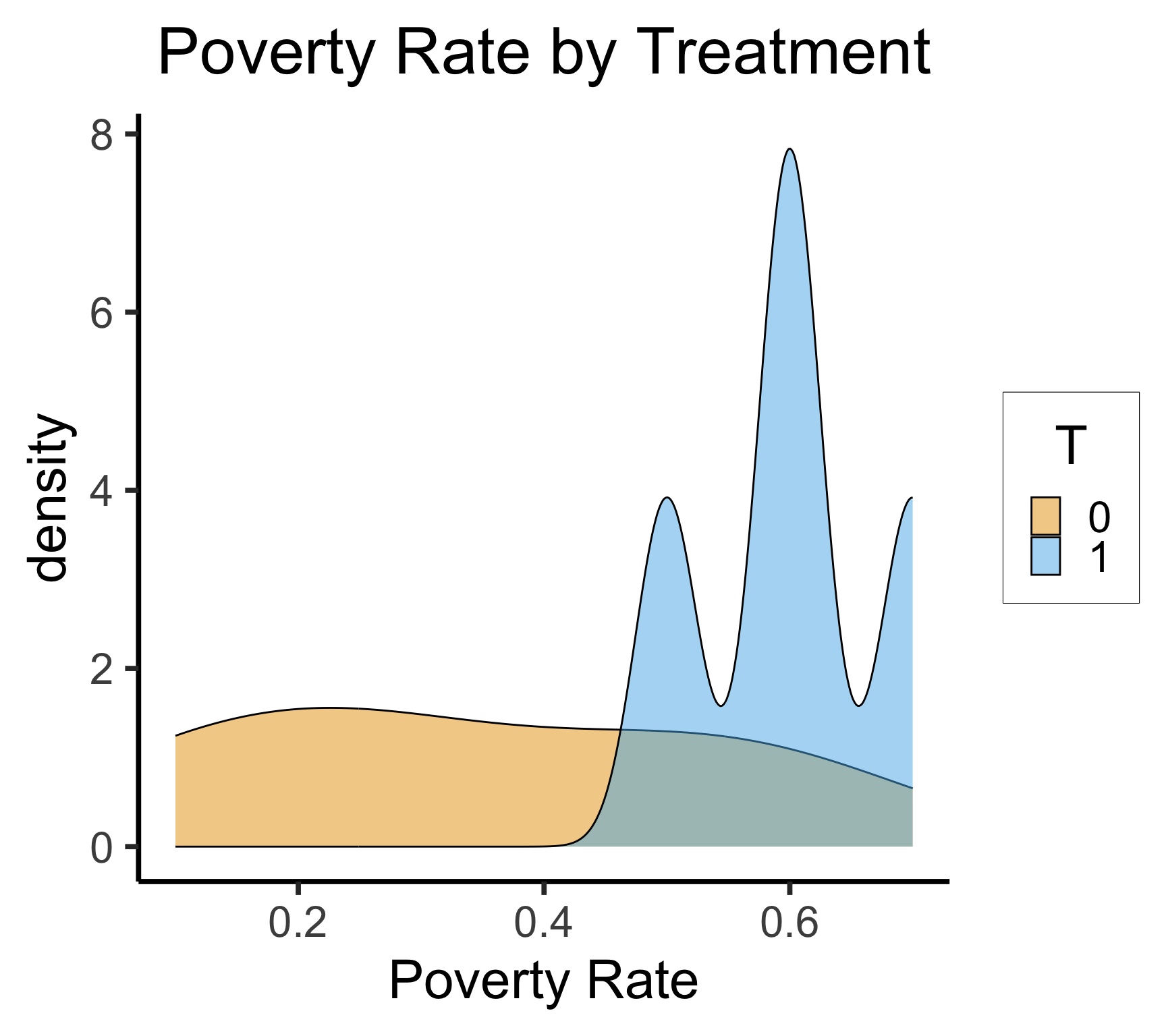
village_df |> ggplot(aes(x = poverty_rate, fill=T)) +
  geom_density(alpha=0.5) +
  theme_dsan(base_size=30) +
  labs(
    title = "Poverty Rate by Treatment",
    x = "Poverty Rate"
  )

Code

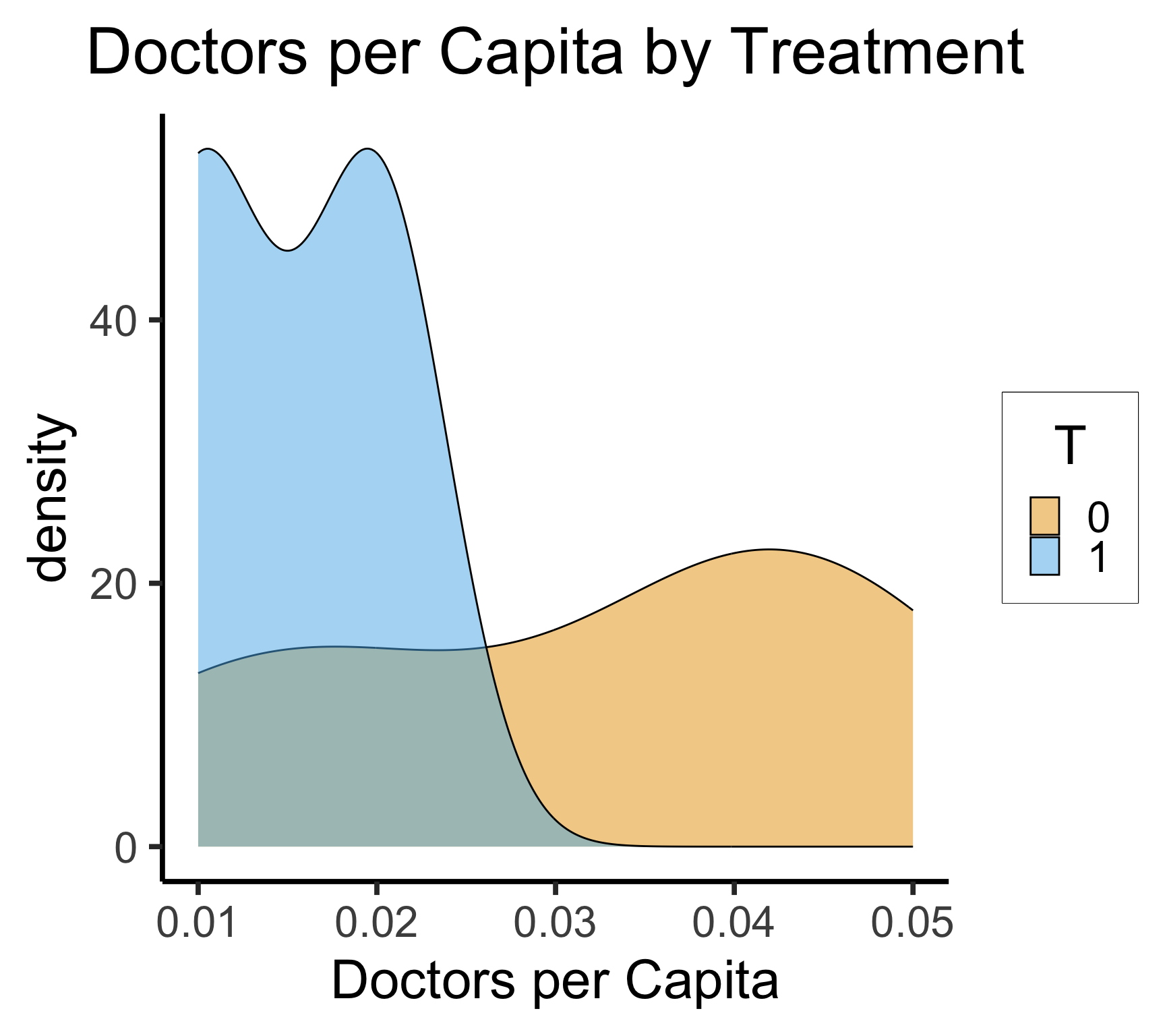
village_df |> ggplot(aes(x = docs_per_capita, fill=T)) +
  geom_density(alpha=0.5) +
  theme_dsan(base_size=30) +
  labs(
    title = "Doctors per Capita by Treatment",
    x = "Doctors per Capita"
  )

\(\leadsto\) We’re not comparing apples to apples! (“Well, we’re both villages”)

Logistic Regression of Treatment

Code

prop_model <- glm(
  T ~ poverty_rate + docs_per_capita,
  data=village_df, family="binomial"
)
summary(prop_model)


Call:
glm(formula = T ~ poverty_rate + docs_per_capita, family = "binomial", 
    data = village_df)

Coefficients:
                Estimate Std. Error z value Pr(>|z|)
(Intercept)       -7.498      8.992  -0.834    0.404
poverty_rate      14.500     13.651   1.062    0.288
docs_per_capita   -8.880    143.595  -0.062    0.951

(Dispersion parameter for binomial family taken to be 1)

    Null deviance: 12.3653  on 8  degrees of freedom
Residual deviance:  6.9987  on 6  degrees of freedom
AIC: 12.999

Number of Fisher Scoring iterations: 6

We now have a model of selection bias! \(\leadsto\) match observations with similar \(\Pr(T)\)

Propensity Score = Logistic Regression Estimate

Code

village_df$ps <- predict(prop_model, village_df, type="response")
village_df

village_id	T	inf_mortality	poverty_rate	docs_per_capita	ps
1	1	10	0.5	0.01	0.4165712
2	1	15	0.6	0.02	0.7358171
3	1	22	0.7	0.01	0.9284516
4	1	19	0.6	0.02	0.7358171
5	0	25	0.6	0.01	0.7527140
6	0	19	0.5	0.02	0.3951619
7	0	4	0.1	0.04	0.0016534
8	0	8	0.3	0.05	0.0268029
9	0	6	0.2	0.04	0.0070107

Propensity Score Matching = Distance Metric!

Code

cur_T <- village_df[1,"T"] |> pull()
cur_ps <- village_df[1,"ps"] |> pull()
writeLines(paste0("Current village: T = ",cur_T,", ps = ",cur_ps))

Current village: T = 1, ps = 0.416571242858422

Code

other_df <- village_df |> filter(T != cur_T) |>
  mutate(
    ps_dist = abs(ps - cur_ps)
  )
other_df |> select(-c(inf_mortality))

village_id	poverty_rate	docs_per_capita	ps	ps_dist
5	0.6	0.01	0.7527140	0.3361428
6	0.5	0.02	0.3951619	0.0214093
7	0.1	0.04	0.0016534	0.4149179
8	0.3	0.05	0.0268029	0.3897683
9	0.2	0.04	0.0070107	0.4095605

Now in a For Loop…

Code

for (i in 1:9) {
  cur_T <- village_df[i,"T"] |> pull()
  cur_ps <- village_df[i,"ps"] |> pull()
  # writeLines(paste0("Current village: T = ",cur_T,", ps = ",cur_ps))
  other_df <- village_df |> filter(T != cur_T) |>
    mutate(
      ps_dist = abs(ps - cur_ps)
    )
  match_id <- names(which.min(other_df$ps_dist))
  village_df[i,"match"] <- as.numeric(match_id)
}
village_df |> select(-inf_mortality)

village_id	T	poverty_rate	docs_per_capita	ps	match
1	1	0.5	0.01	0.4165712	6
2	1	0.6	0.02	0.7358171	5
3	1	0.7	0.01	0.9284516	5
4	1	0.6	0.02	0.7358171	5
5	0	0.6	0.01	0.7527140	2
6	0	0.5	0.02	0.3951619	1
7	0	0.1	0.04	0.0016534	1
8	0	0.3	0.05	0.0268029	1
9	0	0.2	0.04	0.0070107	1

And Now We Compare Apples to Apples…

Code

treated_df <- village_df |> filter(T == 1)
(matched_df <- treated_df |> left_join(village_df, join_by(match == village_id)))

village_id	T.x	inf_mortality.x	poverty_rate.x	docs_per_capita.x	ps.x	match	inf_mortality.y	poverty_rate.y	docs_per_capita.y	ps.y	match.y
1	1	10	0.5	0.01	0.4165712	6	19	0.5	0.02	0.3951619	1
2	1	15	0.6	0.02	0.7358171	5	25	0.6	0.01	0.7527140	2
3	1	22	0.7	0.01	0.9284516	5	25	0.6	0.01	0.7527140	2
4	1	19	0.6	0.02	0.7358171	5	25	0.6	0.01	0.7527140	2

Code

matched_df |> summarize(
  mean_tr = mean(inf_mortality.x),
  mean_control = mean(inf_mortality.y)
)

mean_tr	mean_control
16.5	23.5

\(\leadsto\) Treatment effect \(\approx\) -7 🥳

References

Hume, David. 1739. A Treatise of Human Nature: Being an Attempt to Introduce the Experimental Method of Reasoning Into Moral Subjects; and Dialogues Concerning Natural Religion. Longmans, Green.

Lyall, Jason. 2020. Divided Armies: Inequality and Battlefield Performance in Modern War. Princeton University Press.