Week 6: Regularization for Model Selection
DSAN 5300: Statistical Learning
Spring 2025, Georgetown University
Tuesday, February 18, 2025
Clarification: Target Diagrams
| Low Variance | High Variance | |
|---|---|---|
| Low Bias |  |
 |
| High Bias |  |
 |
Why Was This Helpful for 5100?
- Law of Large Numbers:
- Avg(many sample means \(s\)) \(\leadsto\) true mean \(\mu\)
- \(\widehat{\theta}\) unbiased estimator for \(\theta\):
- Avg(Estimates \(\widehat{\theta}\)) \(\leadsto\) true \(\theta\)
The Low Bias, High Variance case
True Test Error vs. CV Error
Note the icons! Test set = Lake monster: pulling out of water to evaluate kills it 😵
 True Test Error \(\varepsilon_{\text{Test}} = \text{Err}_{\text{Test}}\)
Data \(\mathbf{D}\) “arises” out of (unobservable) DGP
Randomly chop \(\mathbf{D}\) into \(\left[ \mathbf{D}_{\text{Train}} \mid \mathbf{D}_{\text{Test}} \right]\)
\(\underbrace{\text{Err}_{\text{Test}}}_{\substack{\text{Test error,} \\ \text{no cap}}} = f(\mathbf{D}_{\text{Train}} \overset{\text{fit}}{\longrightarrow} \underbrace{\mathcal{M}_{\theta} \overset{\text{eval}}{\longrightarrow} \mathbf{D}_{\text{Test}}}_{\text{This kills monster 😢}})\)
Issue: can only be evaluated once, ever 😱
General Issue with CV: It’s… Halfway There
CV plots will often look like (complexity on \(x\)-axis and CV error on \(y\)-axis):
Code
library(tidyverse) |> suppressPackageStartupMessages()
library(latex2exp) |> suppressPackageStartupMessages()
cpl_label <- TeX("$M_0$")
sim1k_delta_df <- tibble(
    complexity=1:7,
    cv_err=c(8, 2, 1, 1, 1, 1, 2),
    label=c("","",TeX("$M_3$"),"","",TeX("$M_6$"),"")
)
sim1k_delta_df |> ggplot(aes(x=complexity, y=cv_err, label=label)) +
  geom_line(linewidth=1) +
  geom_point(size=(2/3)*g_pointsize) +
  geom_text(vjust=-0.7, size=10, parse=TRUE) +
  scale_x_continuous(
    breaks=seq(from=1,to=7,by=1)
  ) +
  theme_dsan(base_size=22) +
  labs(
    title="Generic CV Error Plot",
    x = "Complexity",
    y = "CV Error"
  )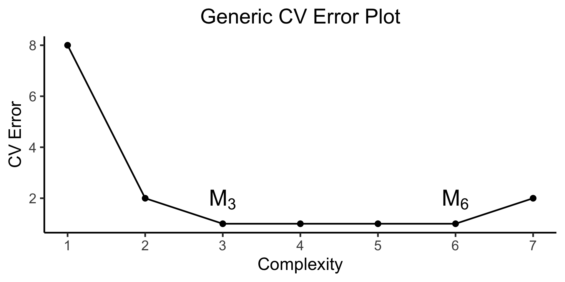
- We “know” \(\mathcal{M}_3\) preferable to \(\mathcal{M}_6\) (same error yet, less overfitting) \(\implies\) “1SE rule”
- But… heuristic \(\;\nimplies\) optimal! What are we gaining/losing as we move \(\mathcal{M}_6 \rightarrow \mathcal{M}_3\)?
- Enter REGULARIZATION!
CV Now Goes Into Your Toolbox

(We will take it back out later, I promise!)
Optimal but Infeasible: Best Subset Selection

Stepwise Selection Algorithms are Greedy
- Like a mouse who chases closest cheese \(\neq\) path with most cheese
- Can get “trapped” in sub-optimal model, if (e.g.) feature is in \(\mathcal{M}^*_4\) but not in \(\mathcal{M}^*_1, \mathcal{M}^*_2, \mathcal{M}^*_3\)!

| \(k\) | \(\mathcal{M}^*_k\) (Best Subset) | \(\mathcal{M}_k\) (Forward Stepwise) |
|---|---|---|
| 1 | rating |
rating |
| 2 | rating, income |
rating, income |
| 3 | rating, income, student |
rating, income, student |
| 4 | cards, income, student, limit |
rating, income, student, limit |
Different Norms \(\leftrightarrow\) Different Distances from \(\vec{\mathbf{0}}\)
- Unit Disk in \(L^2\): All points \(\mathbf{v} = (v_x,v_y) \in \mathbb{R}^2\) such that
\[ \| \mathbf{v} \|_2 \leq 1 \iff \| \mathbf{v} \|_2^2 \leq 1 \]

- Unit Disk in \(L^1\): All points \(\mathbf{v} = (v_x, v_y) \in \mathbf{R}^2\) such that
\[ \| \mathbf{v} \|_1 \leq 1 \]

The Key Plot
Code
library(tidyverse) |> suppressPackageStartupMessages()
library(latex2exp) |> suppressPackageStartupMessages()
library(ggforce) |> suppressPackageStartupMessages()
library(patchwork) |> suppressPackageStartupMessages()
# Bounding the space
xbound <- c(-1, 1)
ybound <- c(0, 1.65)
stepsize <- 0.05
dx <- 0.605
dy <- 1.6
# The actual function we're plotting contours for
b_inter <- 1.5
my_f <- function(x,y) 8^(b_inter*(x-dx)*(y-dy) - (x-dx)^2 - (y-dy)^2)
x_vals <- seq(from=xbound[1], to=xbound[2], by=stepsize)
y_vals <- seq(from=ybound[1], to=ybound[2], by=stepsize)
data_df <- expand_grid(x=x_vals, y=y_vals)
data_df <- data_df |> mutate(
  z = my_f(x, y)
)
# Optimal beta df
beta_opt_df <- tibble(
  x=121/200, y=8/5, label=c(TeX("$\\beta^*_{OLS}$"))
)
# Ridge optimal beta
ridge_opt_df <- tibble(
  x=0.111, y=0.998, label=c(TeX("$\\beta^*_{ridge}$"))
)
# Lasso diamond
lasso_df <- tibble(x=c(1,0,-1,0,1), y=c(0,1,0,-1,0), z=c(1,1,1,1,1))
lasso_opt_df <- tibble(x=0, y=1, label=c(TeX("$\\beta^*_{lasso}$")))

# And plot
base_plot <- ggplot() +
  geom_contour_filled(
    data=data_df, aes(x=x, y=y, z=z),
    alpha=0.8, binwidth = 0.04, color='black', linewidth=0.65
  ) +
  # y-axis
  geom_segment(aes(x=0, xend=0, y=-Inf, yend=Inf), color='white', linewidth=0.5, linetype="solid") +
  # Unconstrained optimal beta
  geom_point(data=beta_opt_df, aes(x=x, y=y), size=2) +
  geom_label(
    data=beta_opt_df, aes(x=x, y=y, label=label),
    hjust=-0.45, vjust=0.65, parse=TRUE, alpha=0.9
  ) +
  scale_fill_viridis_d(option="C") +
  #coord_equal() +
  labs(
    #title = "Model Selection: Ridge vs. Lasso Constraints",
    x = TeX("$\\beta_1$"),
    y = TeX("$\\beta_2$")
  )
ridge_plot <- base_plot +
  geom_circle(
    aes(x0=0, y0=0, r=1, alpha=I(0.1), linetype="circ", color='circ'), fill=NA, linewidth=0.5
  )
  # geom_point(
  #   data=data.frame(x=0, y=0), aes(x=x, y=y),
  #   shape=21, size=135.8, color='white', stroke=1.2, linestyle="dashed"
  # )
lasso_plot <- ridge_plot +
  geom_polygon(
    data=lasso_df, aes(x=x, y=y, linetype="diamond", color="diamond"),
    fill='white',
    alpha=0.5,
    linewidth=1
  ) +
  # Ridge beta
  geom_point(data=ridge_opt_df, aes(x=x, y=y), size=2) +
  geom_label(
    data=ridge_opt_df, aes(x=x, y=y, label=label),
    hjust=2, vjust=-0.15, parse=TRUE, alpha=0.9
  ) +
  # Lasso beta
  geom_point(data=lasso_opt_df, aes(x=x, y=y), size=2) +
  geom_label(
    data=lasso_opt_df, aes(x=x, y=y, label=label),
    hjust=-0.75, vjust=-0.15, parse=TRUE, alpha=0.9
  ) +
  ylim(ybound[1], ybound[2]) +
  # xlim(xbound[1], xbound[2]) +
  scale_linetype_manual("Line", values=c("diamond"="solid", "circ"="dashed"), labels=c("a","b")) +
  scale_color_manual("Color", values=c("diamond"="white", "circ"="white"), labels=c("c","d")) +
  # scale_fill_manual("Test") +
  # x-axis
  geom_segment(aes(x=-Inf, xend=Inf, y=0, yend=0), color='white') +
  theme_dsan(base_size=16) +
  coord_fixed() +
  theme(
    legend.position = "none",
    axis.line = element_blank(),
    axis.ticks = element_blank()
  )
lasso_plot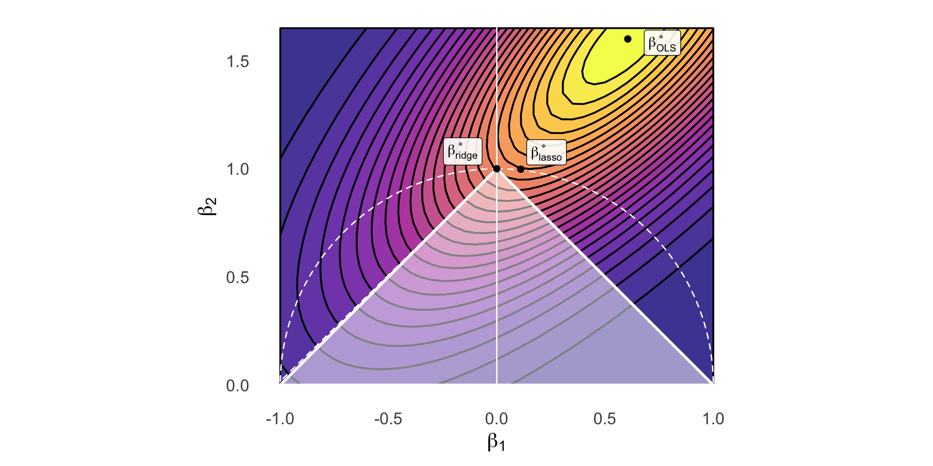
Bayesian Interpretation
- Belief \(A\): Most/all of the features you included have important effect on \(Y\)
- \(A \implies\) Gaussian prior on \(\beta_j\), \(\mu = 0\)
- If \(X \sim \mathcal{N}(\mu, \sigma^2)\), pdf of \(X\) is
\[ f_X(x) = \frac{1}{\sqrt{2\pi \sigma^2}}\exp\left[ -\frac{1}{2}\left( \frac{x-\mu}{\sigma}\right)^2 \right] \]
Code
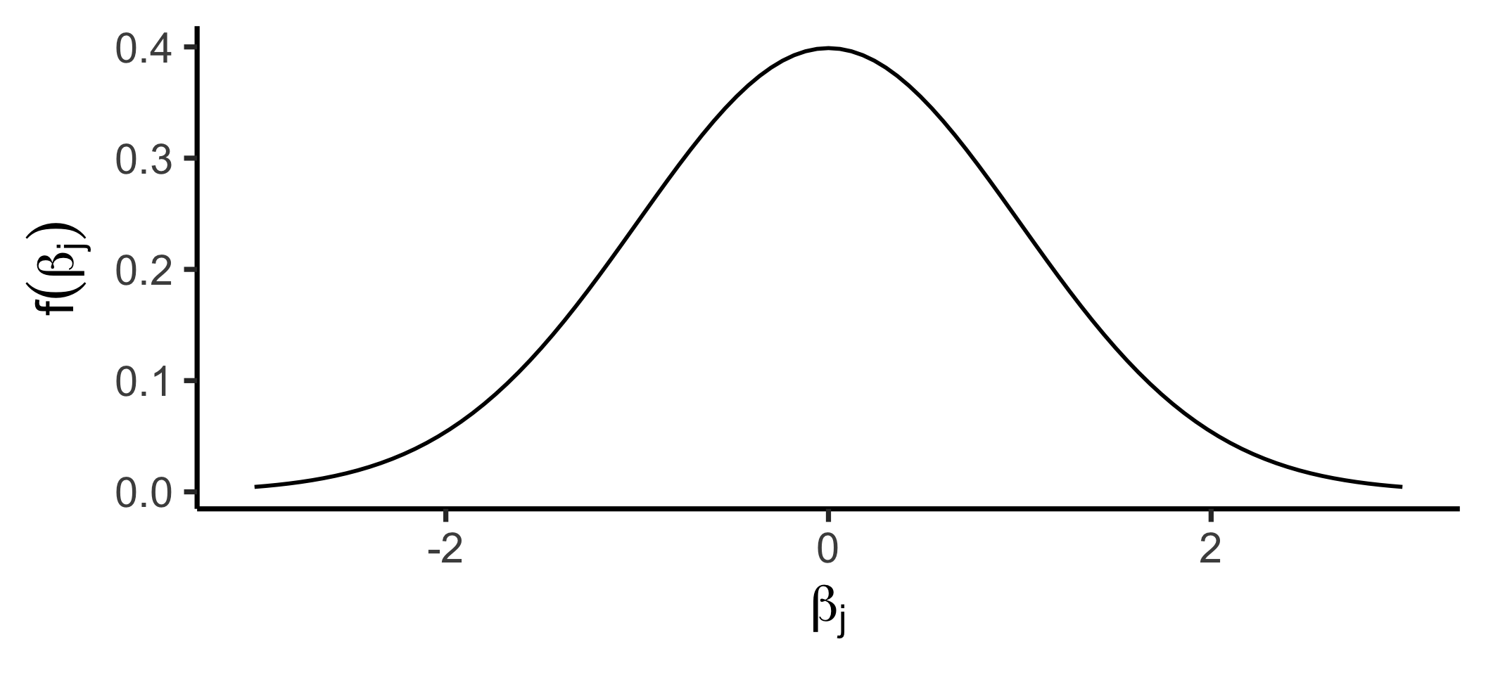
- Gaussian prior \(\leadsto\) Ridge Regression!
(High complexity penalty \(\lambda\) \(\leftrightarrow\) low \(\sigma^2\))
- Belief \(B\): Only a few of the features you included have important effect on \(Y\)
- \(B \implies\) Laplacian prior on \(\beta_j\), \(\mu = 0\)
- If \(X \sim \mathcal{L}(\mu, b)\), pdf of \(X\) is
\[ f(x) = \frac{1}{2b}\exp\left[ -\left| \frac{x - \mu}{b} \right| \right] \]
Code
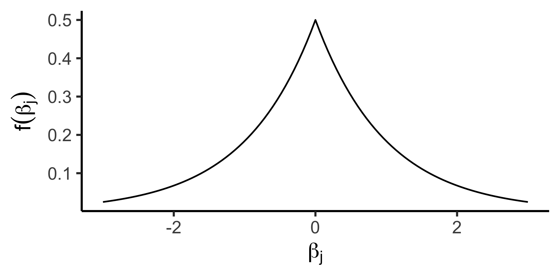
- Laplacian prior \(\leadsto\) Lasso!
(High complexity penalty \(\lambda\) \(\leftrightarrow\) low \(b\))
Varying \(\lambda\) \(\leadsto\) Tradeoff Curve!

Only Change: \(L^1\) instead of \(L^2\) Norm 🤯

Week 7 Preview: Linear Functions
- You’ve already seen polynomial regression:
\[ Y = \beta_0 + \beta_1X + \beta_2X^2 + \beta_3X^3 + \cdots + \beta_d X^d \]
- Plus (technically) “Fourier regression”:
\[ \begin{align*} Y = \beta_0 + \beta_1 \cos(\pi X) + \beta_2 \sin(\pi X) + \cdots + \beta_{2d-1}\cos(\pi d X) + \beta_{2d}\sin(\pi d X) \end{align*} \]

New Regression Just Dropped
Piecewise regression:
Choose \(K\) cutpoints \(c_1, \ldots, c_K\)
Let \(C_k(X) = \mathbb{1}[c_{k-1} \leq X < c_k]\), (\(c_0 \equiv -\infty\), \(c_{K+1} \equiv \infty\))
\[ Y = \beta_0 + \beta_1C_1(X) + \beta_2C_2(X) + \cdots + \beta_KC_K(X) \]
