This document contains clarifications for the Lab 6 assignment, based on details and/or hints that I’ve found helpful during office hours and email discussions about the assignment!
Images and Assignment Files
For the core assignment that you’ll need to complete, please make sure that you download:
The Lab6_assignment.qmd file, as well as
The images folder,
and make sure to download these into the same directory. For example, I usually have a directory on my laptop structured so that I can download each assignment into its own subfolder within a folder called dsan5100, so that the path to the .qmd file looks something like (this is the partial output from running tree dsan5100):
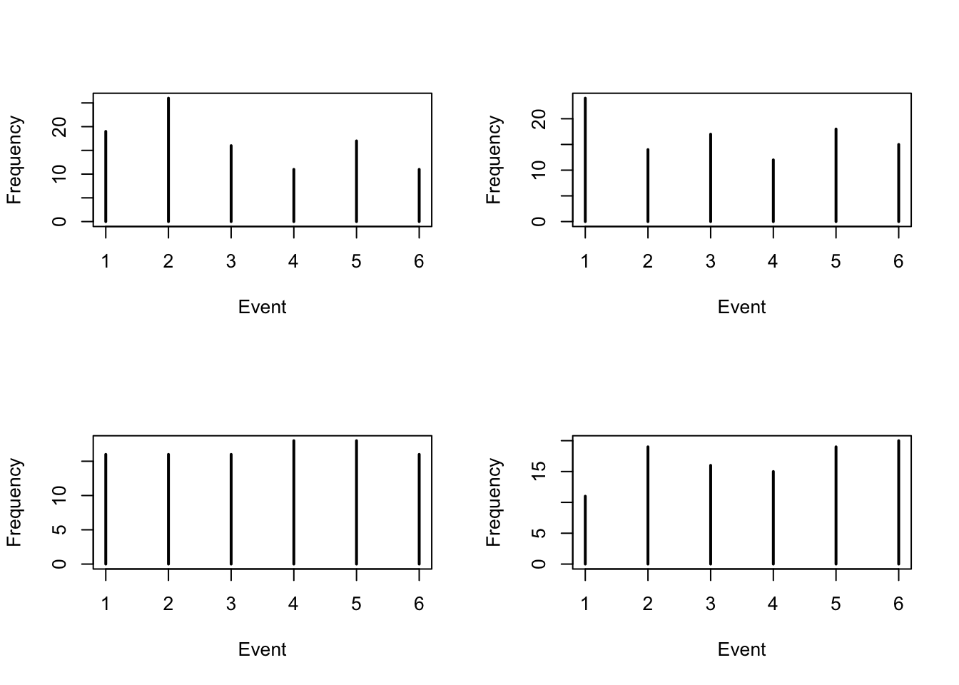
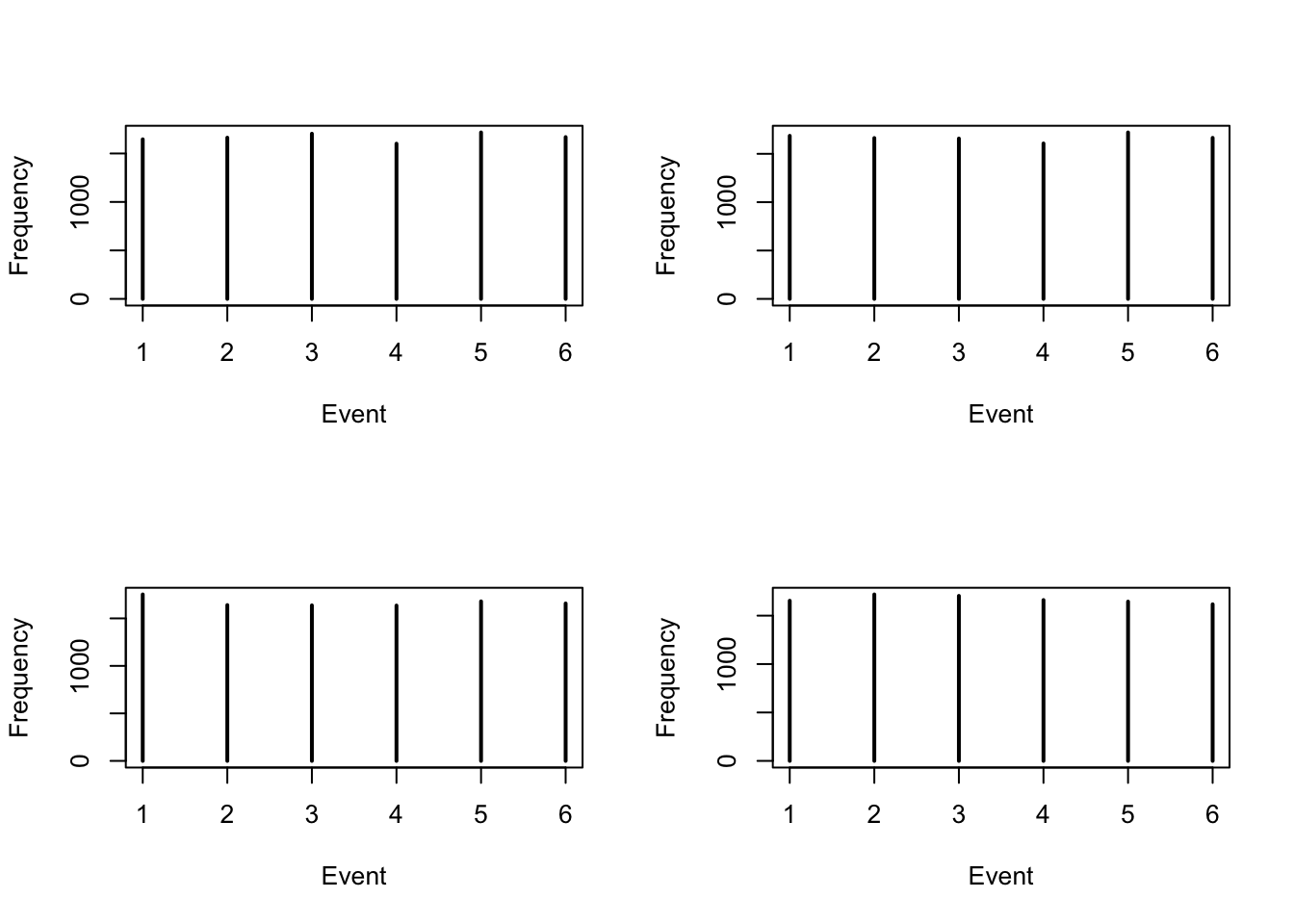
The following code is the same as the code in the Lab assignment, but here we seed the random number generator so it produces the same exact results every time it is run. (This makes it easier to refer to “the” plots in the problem, when helping in office hours: using set.seed(5100) ensures that the plots are the same between students’ and teachers’ computers!)
Since the “Shopping Example” image displays kind of fuzzily, on my screen at least, here is the problem (including the image) just re-written to use HTML rather than image files:
Shopping Example
Suppose there are two types of items [My understanding is that this should be three types of items] and \(n = 3\) customers.
Possible values are \(\{(3,0,0),(2,1,0),(2,0,1), \ldots, (0,1,2), (0,0,3)\}\)
Some values of the joint pmf:
\(\Pr((3,0,0)) = 1 \cdot (p_1)^3\)
\(\Pr((1,2,0)) = 3 \cdot (p_1)(p_2)^2\)
\(\Pr((1,1,1)) = 6 \cdot (p_1)(p_2)(p_3)\)
(The factors 1, 3, 6 count the number of ways in which these events can occur)
Table 1: The example table given in the image, showing
Beer
Bread
Coke
3
0
0
2
1
0
2
0
1
0
3
0
0
2
1
0
1
2
1
0
2
1
2
0
1
1
1
0
0
3
Let’s say that Molly, Ryan, and Mr. Bob are buying Beer (\(X_1\)), Bread (\(X_2\)), and Coke (\(X_3\)) with probabilities \(\left(3/5, 1/5, 1/5\right)\).
What is the probability that only one of them will buy Beer, two of them will buy Bread, and none of them will buy Coke? Compare the result with the theoretical probability.
Do a simulation for this scenario and plot the marginal distribution of \(X_1\).
Problem 3
Here, from what I understand, the problem letters jump from (c) to (e), so that there is no Part (d) for Problem 3.