Although a discrete distribution is characterized by its PMF and a continuous distribution is characterized by its PDF, every distribution has a common characterization through its (cumulative) distribution function (CDF). The inverse of the CDF is called the quantile function, and it is useful for indicating where the probability is located in a distribution.
It should be emphasized that the cumulative distribution function is defined as above for every random variable X, regardless of whether the distribution of X is discrete, continuous, or mixed. For the continuous random variable in Example 3.3.1, the CDF was calculated in eq-3-3-1. Here is a discrete example:
We shall soon see (Theorem 3.3.2) that the CDF allows calculation of all interval probabilities; hence, it characterizes the distribution of a random variable. It follows from eq-3-3-2 that the CDF of each random variable X is a function F defined on the real line. The value of F at every point x must be a number F(x) in the interval [0,1] because F(x) is the probability of the event {X≤x}. Furthermore, it follows from eq-3-3-2 that the CDF of every random variable X must have the following three properties.
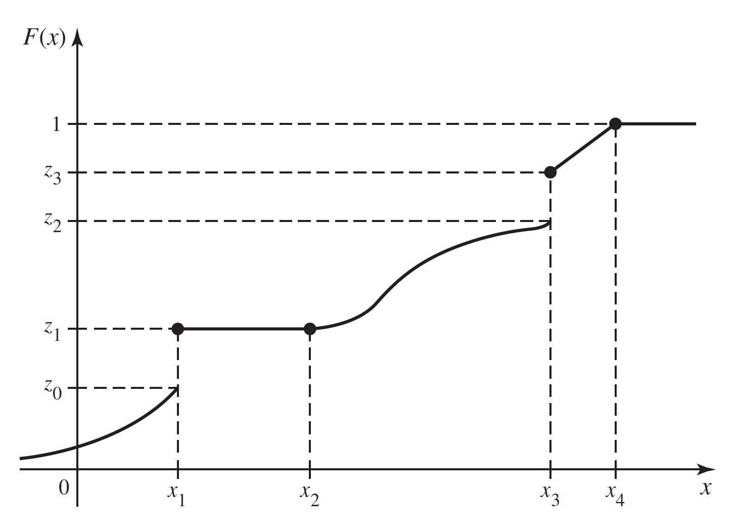
An example of a CDF is sketched in Figure 3.6. It is shown in that figure that 0≤F(x)≤1 over the entire real line. Also, F(x) is always nondecreasing as x increases, although F(x) is constant over the interval x1≤x≤x2 and for x≥x4.
The limiting values specified in Property 3.3.2 are indicated in Figure 3.6. In this figure, the value of F(x) actually becomes 1 at x=x4 and then remains 1 for x>x4. Hence, it may be concluded that Pr(X≤x4)=1 and Pr(X>x4)=0. On the other hand, according to the sketch in Figure 3.6, the value of F(x) approaches 0 as x→−∞, but does not actually become 0 at any finite point x. Therefore, for every finite value of x, no matter how small, Pr(X≤x)>0.
A CDF need not be continuous. In fact, the value of F(x) may jump at any finite or countable number of points. In Figure 3.6, for instance, such jumps or points of discontinuity occur where x=x1 and x=x3. For each fixed value x, we shall let F(x−) denote the limit of the values of F(y) as y approaches x from the left, that is, as y approaches x through values smaller than x. In symbols,
In Figure 3.6 this property is illustrated by the fact that, at the points of discontinuity x=x1 and x=x3, the value of F(x1) is taken as z1 and the value of F(x3) is taken as z3.
Determining Probabilities from the Distribution Function
The type of reasoning used in Example 3.3.3 can be extended to find the probability that an arbitrary random variable X will lie in any specified interval of the real line from the CDF. We shall derive this probability for four different types of intervals.
For example, if the CDF of X is as sketched in Figure 3.6, then it follows from Theorems Theorem 3.3.1 and Theorem 3.3.2 that Pr(X>x2)=1−z1 and Pr(x2<X≤x3)=z3−z1. Also, since F(x) is constant over the interval x1≤x≤x2, then Pr(x1<X≤x2)=0.
It is important to distinguish carefully between the strict inequalities and the weak inequalities that appear in all of the preceding relations and also in the next theorem. If there is a jump in F(x) at a given value x, then the values of Pr(X≤x) and Pr(X<x) will be different.
For example, for the CDF sketched in Figure 3.6, Pr(X<x3)=z2 and Pr(X<x4)=1.
Finally, we shall show that for every value x, Pr(X=x) is equal to the amount of the jump that occurs in F at the point x. If F is continuous at the point x, that is, if there is no jump in F at x, then Pr(X=x)=0.
In Figure 3.6, for example, Pr(X=x1)=z1−z0, Pr(X=x3)=z3−z2, and the probability of every other individual value of X is 0.
From the definition and properties of a CDF F(x), it follows that if a<b and if Pr(a<X<b)=0, then F(x) will be constant and horizontal over the interval a<x<b. Furthermore, as we have just seen, at every point x such that Pr(X=x)>0, the CDF will jump by the amount Pr(X=x).
Suppose that X has a discrete distribution with the pmf f(x). Together, the properties of a CDF imply that F(x) must have the following form: F(x) will have a jump of magnitude f(xi) at each possible value xi of X, and F(x) will be constant between every pair of successive jumps. The distribution of a discrete random variable X can be represented equally well by either the pmf or the CDF of X.
Thus, the CDF of a continuous random variable X can be obtained from the pdf and vice versa. eq-3-3-7 is how we found the CDF in Example 3.3.1. Notice that the derivative of the F in Example 3.3.1 is
and F′ does not exist at x=0. This verifies eq-3-3-8 for Example 3.3.1. Here, we have used the popular shorthand notation F′(x) for the derivative of F at the point x.
The value x0 that we seek in Example 3.3.5 is called the 0.5 quantile of X or the 50th percentile of X because 50% of the distribution of X is at or below x0.
The notation F−1(p) in Definition 3.3.2 deserves some justification. Suppose first that the CDF F of X is continuous and one-to-one over the whole set of possible values of X. Then the inverse F−1 of F exists, and for each 0<p<1, there is one and only one x such that F(x)=p. That x is F−1(p). Definition 3.3.2 extends the concept of inverse function to nondecreasing functions (such as CDFs) that may be neither one-to-one nor continuous.
Quantiles of Continuous Distributions: When the CDF of a random variable X is continuous and one-to-one over the whole set of possible values of X, the inverse F−1 of F exists and equals the quantile function of X.
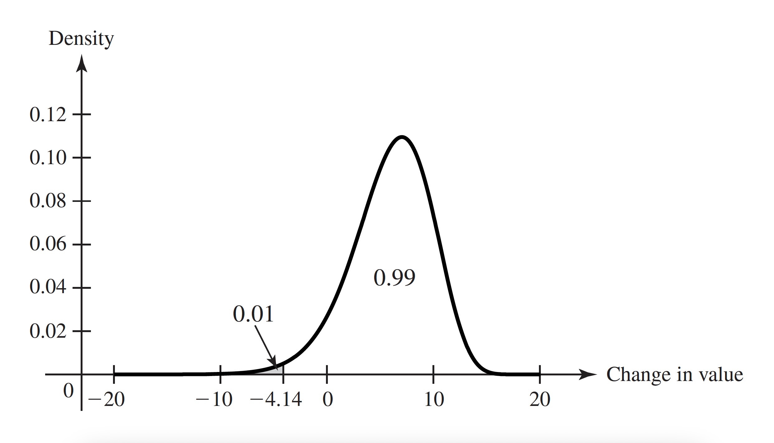
Figure 3.7:The pdf of the change in value of a portfolio with lower 1% indicated
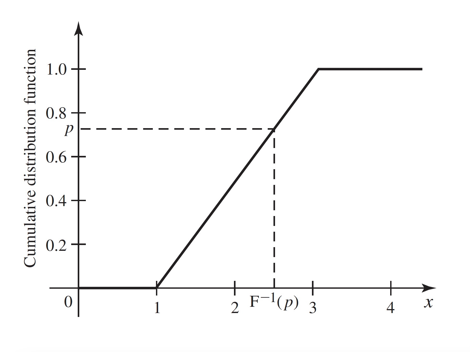
Figure 3.8:The CDF of a uniform distribution indicating how to solve for a quantile
Note: Quantiles, Like CDFs, Depend on the Distribution Only: Any two random variables with the same distribution have the same quantile function. When we refer to a quantile of X, we mean a quantile of the distribution of X.
Quantiles of Discrete Distributions: It is convenient to be able to calculate quantiles for discrete distributions as well. The quantile function of Definition 3.3.2 exists for all distributions whether discrete, continuous, or otherwise. For example, in Figure 3.6, let z0≤p≤z1. Then the smallest x such that F(x)≥p is x1. For every value of x<x1, we have F(x)<z0≤p and F(x1)=z1. Notice that F(x)=z1 for all x between x1 and x2, but since x1 is the smallest of all those numbers, x1 is the p quantile. Because distribution functions are continuous from the right, the smallest x such that F(x)≥p exists for all 0<p<1. For p=1, there is no guarantee that such an x will exist. For example, in Figure 3.6, F(x4)=1, but in Example 3.3.1, F(x)<1 for all x. For p=0, there is never a smallest x such that F(x)=0 because limx→−∞F(x)=0. That is, if F(x0)=0, then F(x)=0 for all x<x0. For these reasons, we never talk about the 0 or 1 quantiles.
p
F−1(p)
(0,0.1681]
0
(0.1681,0.5283]
1
(0.5283,0.8370]
2
(0.8370,0.9693]
3
(0.9693,0.9977]
4
(0.9977,1)
5
: Table 3.1: Quantile function for Example 3.3.9. {#tbl-3-1}
The median of a distribution is one of several special features that people like to use when sumarizing the distribution of a random variable. We shall discuss summaries of distributions in more detail in Chapter 4: Expectation. Because the median is such a popular summary, we need to note that there are several different but similar “definitions” of median. Recall that the 1/2 quantile is the smallest number x such that F(x)≥1/2. For some distributions, usually discrete distributions, there will be an interval of numbers [x1,x2) such that for all x∈[x1,x2), F(x)=1/2. In such cases, it is common to refer to all such x (including x2) as medians of the distribution. (See Definition 4.5.1.) Another popular convention is to call (x1+x2)/2 the median. This last is probably the most common convention. The readers should be aware that, whenever they encounter a median, it might be any one of the things that we just discussed. Fortunately, they all mean nearly the same thing, namely that the number divides the distribution in half as closely as is possible.
One advantage to describing a distribution by the quantile function rather than by the CDF is that quantile functions are easier to display in tabular form for multiple distributions. The reason is that the domain of the quantile function is always the interval (0,1) no matter what the possible values of X are. Quantiles are also useful for summarizing distributions in terms of where the probability is. For example, if one wishes to say where the middle half of a distribution is, one can say that it lies between the 0.25 quantile and the 0.75 quantile. In sec-8-5, we shall see how to use quantiles to help provide estimates of unknown quantities after observing data.
In Div, you can show how to recover the CDF from the quantile function. Hence, the quantile function is an alternative way to characterize a distribution.
The CDF F of a random variable X is F(x)=Pr(X≤x) for all real x. This function is continuous from the right. If we let F(x−) equal the limit of F(y) as y approaches x from below, then F(x)−F(x−)=Pr(X=x). A continuous distribution has a continuous CDF and F′(x)=f(x), the pdf of the distribution, for all x at which F is differentiable. A discrete distribution has a CDF that is constant between the possible values and jumps by f(x) at each possible value x. The quantile function F−1(p) is equal to the smallest x such that F(x)≥p for 0<p<1.
Suppose that a random variable X can take only the values −2, 0, 1, and 4, and that the probabilities of these values are as follows: Pr(X=−2)=0.4, Pr(X=0)=0.1, Pr(X=1)=0.3, and Pr(X=4)=0.2. Sketch the CDF of X.
Suppose that a coin is tossed repeatedly until a head is obtained for the first time, and let X denote the number of tosses that are required. Sketch the CDF of X.
Suppose that a point in the xy-plane is chosen at random from the interior of a circle for which the equation is x2+y2=1; and suppose that the probability that the point will belong to each region inside the circle is proportional to the area of that region. Let Z denote a random variable representing the distance from the center of the circle to the point. Find and sketch the CDF of Z.
Suppose that X has the uniform distribution on the interval [0,5] and that the random variable Y is defined by Y=0 if X≤1, Y=5 if X≥3, and Y=X otherwise. Sketch the CDF of Y.
Suppose that a broker believes that the change in value X of a particular investment over the next two months has the uniform distribution on the interval [−12,24]. Find the value at risk VaR for two months at probability level 0.95.
Prove that the quantile function F^{-1} of a general random variable X has the following three properties that are analogous to properties of the CDF:
a. F−1 is a nondecreasing function of p for 0<p<1.
b. Let x0=limp→0,p>0F−1(p) and x1=limp→1,p<1F−1(p). Then x0 equals the greatest lower bound on the set of numbers c such that Pr(X≤c)>0, and x1 equals the least upper bound on the set of numbers d such that Pr(X≥d)>0.
c. F−1 is continuous from the left; that is F−1(p)=F−1(p−) for all 0<p<1.
Let X be a random variable with quantile function F−1. Assume the following three conditions: (i) F−1(p)=c for all p in the interval (p0,p1), (ii) either p0=0 or F−1(p0)<c, and (iii) either p1=1 or F−1(p)>c for p>p1. Prove that Pr(X=c)=p1−p0.
Let X be a random variable with CDF F and quantile function F−1. Let x0 and x1 be as defined in Div. (Note that x0=−∞and/orx_1 = \inftyarepossible.)Provethatforallxintheopeninterval(x_0, x_1),F(x)isthelargestpsuchthatF^{−1}(p) \leq x$.