Overview
We generalize the concept of distribution of a random variable to the joint distribution of two random variables. In doing so, we introduce the joint pmf for two discrete random variables, the joint pdf for two continuous random variables, and the joint CDF for any two random variables. We also introduce a joint hybrid of pmf and pdf for the case of one discrete random variable and one continuous random variable.
It is a straightforward consequence of the definition of the joint distribution of and that this joint distribution is itself a probability measure on the set of ordered pairs of real numbers. The set will be an event for every set of pairs of real numbers that most readers will be able to imagine.
In this section and the next two sections, we shall discuss convenient ways to characterize and do computations with bivariate distributions. In 3.7 Multivariate Distributions, these considerations will be extended to the joint distribution of an arbitrary finite number of random variables.
3.4.1 Discrete Joint Distributions
The two random variables in Example 3.4.2 have a discrete joint distribution.
When we define continuous joint distribution shortly, we shall see that the obvious analog of Theorem 3.4.1 is not true.
The following result is easy to prove because there are at most countably many pairs that must account for all of the probability a discrete joint distribution.
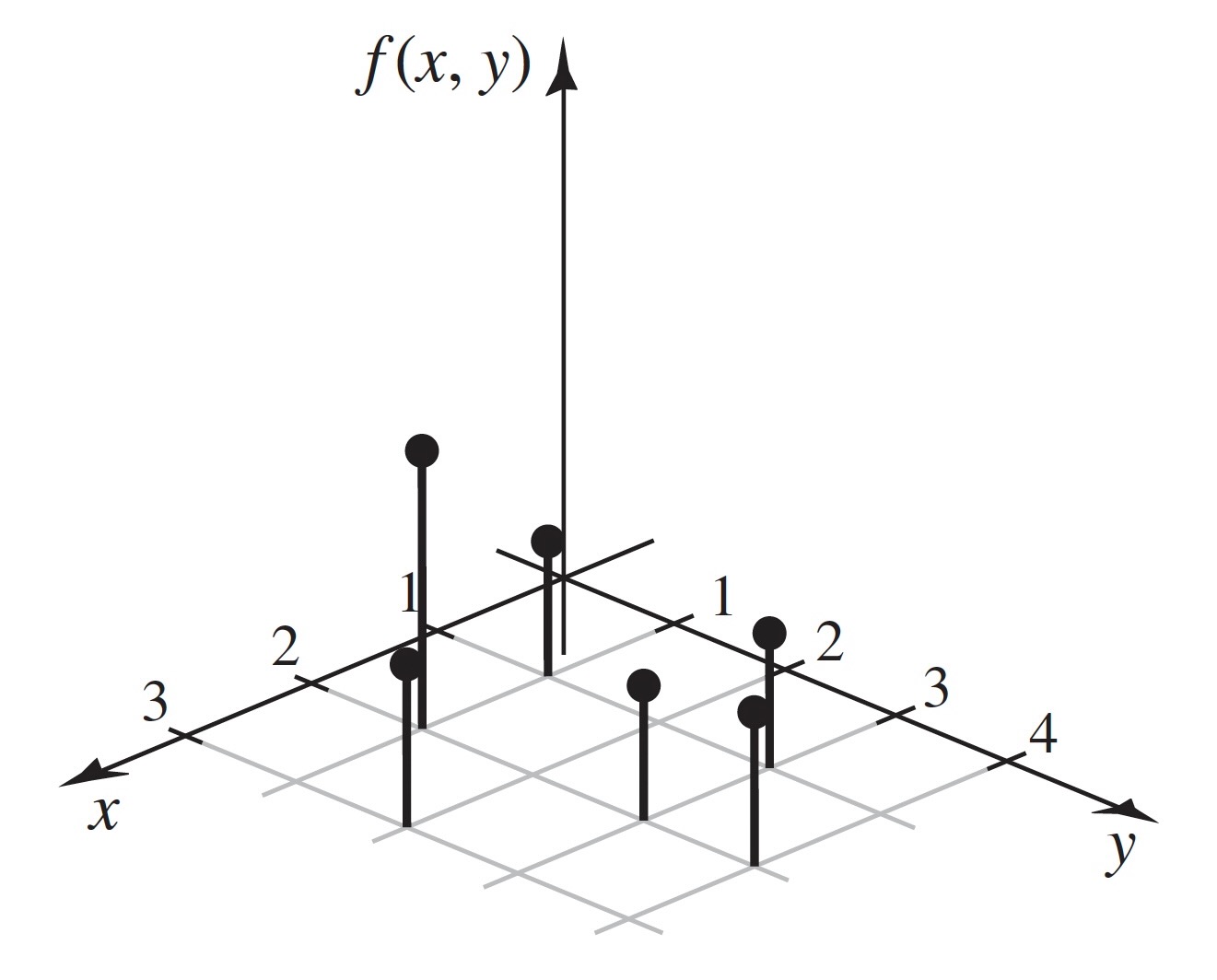
Figure 3.10:The joint pmf of and in Example 3.4.3
Continuous Joint Distributions
If one looks carefully at (3.4.1), one will notice the similarity to (3.2.2) and (3.2.1). We formalize this connection as follows.
It is clear from Definition 3.4.4 that the joint pdf of two random variables characterizes their joint distribution. The following result is also straightforward.
Any function that satisfies the two displayed formulas in Theorem 3.4.3 is the joint pdf for some probability distribution.
An example of the graph of a joint pdf is presented in Figure 3.11.
The total volume beneath the surface and above the -plane must be 1. The probability that the pair will belong to the rectangle is equal to the volume of the solid figure with base shown in Figure 3.11. The top of this solid figure is formed by the surface .
In 3.5 Marginal Distributions, we will show that if and have a continuous joint distribution, then and each have a continuous distribution when considered separately. This seems reasonable intutively. However, the converse of this statement is not true, and the following result helps to show why.
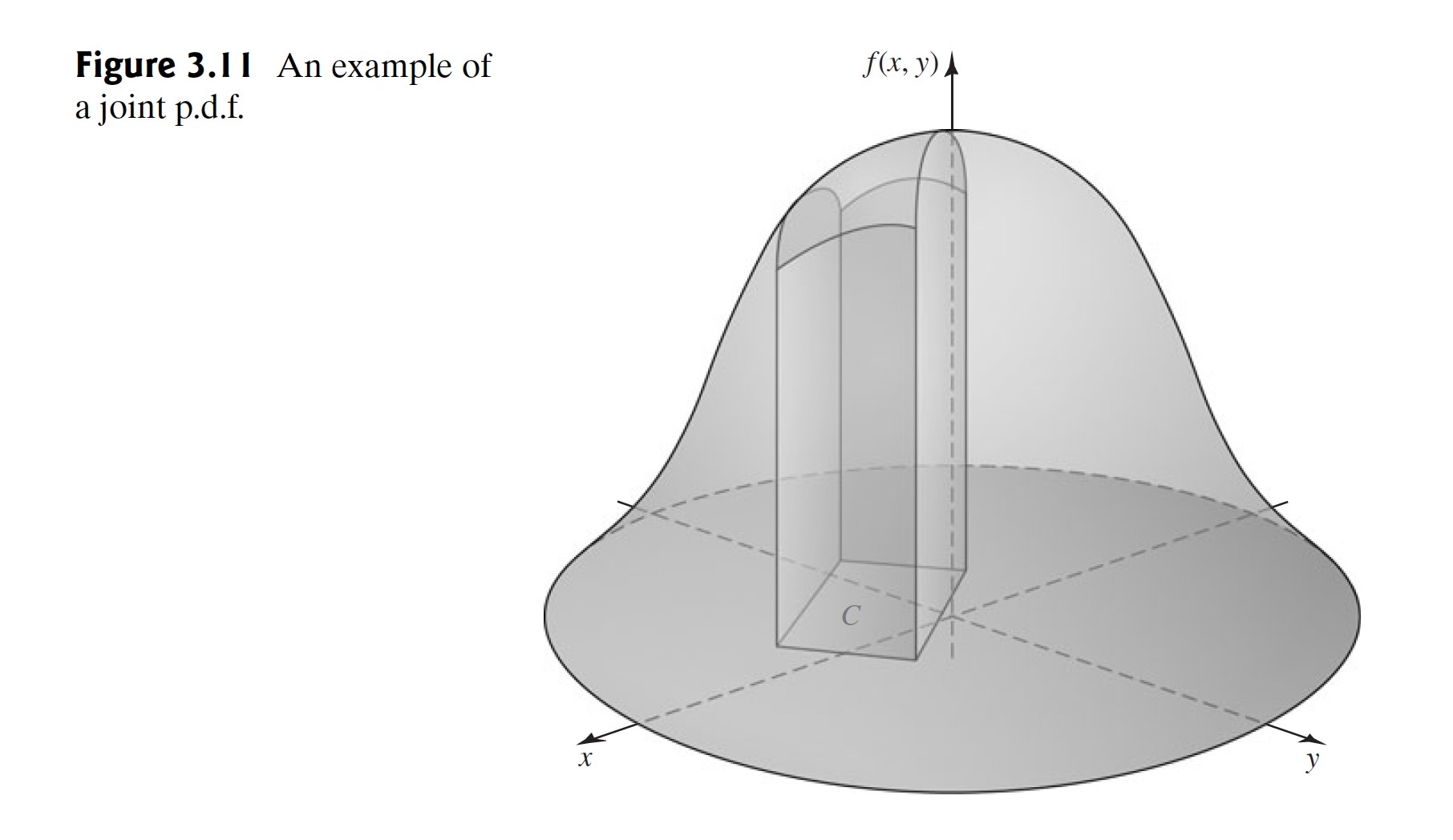
Figure 3.11:An example of a joint pdf
{#fig-3-12}
{#fig-3-13}
::: {.callout-tip title="Example 3.4.9"}
::: {#exm-3-4-9}
# Example 3.4.9: Determining a Joint pdf by Geometric Methods.
Suppose that a point $(X, Y)$ is selected at random from inside the circle $x^2 + y^2 \leq 9$. We shall determine the joint pdf of $X$ and $Y$.
The support of $(X, Y)$ is the set $S$ of points on and inside the circle $x^2 + y^2 \leq 9$. The statement that the point $(X, Y)$ is selected at random from inside the circle is interpreted to mean that the joint pdf of $X$ and $Y$ is constant over $S$ and is 0 outside $S$. Thus,
$$
f(x, y) = \begin{cases}
c &\text{for }(x, y) \in S, \\
0 &\text{otherwise.}
\end{cases}
$$
We must have
$$
\int_{S}\int f(x, y) \, dx \, dy = c \times \text{(area of }S\text{)} = 1.
$$
Since the area of the circle $S$ is $9\pi$, the value of the constant $c$ must be $1/(9\pi)$.
(sec-3-4-3)=
# Mixed Bivariate Distributions

::: {.callout-tip title="Example 3.4.10"}
::: {#exm-3-4-10}

# Example 3.4.10: A Clinical Trial

Consider a clinical trial (such as the one described in @exm-2-1-12) in which each patient with depression receives a treatment and is followed to see whether they have a relapse into depression. Let $X$ be the indicator of whether or not the first patient is a "success" (no relapse). That is $X = 1$ if the patient does not relapse and $X = 0$ if the patient relapses. Also, let $P$ be the proportion of patients who have no replapse among all patients who might receive the treatment. It is clear that $X$ must have a discrete distribution, but it might be sensible to think of $P$ as a continuous random variable taking its value anywhere in the interval $[0, 1]$. Even though $X$ and $P$ can have neither a joint discrete distribution nor a joint continuous distribution, we can still be interested in the joint distribution of $X$ and $P$.
Prior to @exm-3-4-10, we have discussed bivariate distributions that were either discrete or continuous. Occasionally, one must consider a mixed bivariate distribution in which one of the random variables is discrete and the other is continuous. We shall use a function $f(x, y)$ to characterize such a joint distribution in much the
same way that we use a joint pmf to characterize a discrete joint distribution or a joint pdf to characterize a continuous joint distribution.

::: {.callout-note title="Definition 3.4.5"}
::: {#def-3-4-5}

# Definition 3.4.5: Joint pmf/pdf

Let $X$ and $Y$ be random variables such that $X$ is discrete and $Y$ is continuous. Suppose that there is a function $f(x, y)$ defined on the $xy$-plane such that, for every pair $A$ and $B$ of subsets of the real numbers,

$$
\Pr(X \in A \text{ and } Y \in B) = \int_{B}\sum_{x \in A}f(x,y) \, dy,
$$ {#eq-3-4-4}

if the integral exists. Then the function $f$ is called the *joint pmf/pdf* of $X$ and $Y$.
Clearly, @def-3-4-5 can be modified in an obvious way if $Y$ is discrete and $X$ is continuous. Every joint pmf/pdf must satisfy two conditions. If $X$ is the discrete random variable with possible values $x_1, x_2, \ldots$ and $Y$ is the continuous random variable, then $f(x, y) \geq 0$ for all $x$, $y$ and

$$
\int_{-\infty}^{\infty}\sum_{i=1}^{\infty} f(x_i, y) \, dy = 1.
$$ {#eq-3-4-5}

Because $f$ is nonnegative, the sum and integral in Eqs. [-@eq-3-4-4] and [-@eq-3-4-5] can be done in whichever order is more convenient.

**Note: Probabilities of More General Sets.** For a general set $C$ of pairs of real numbers, we can compute $\Pr((X, Y) \in C)$ using the joint pmf/pdf of $X$ and $Y$. For each $x$, let $C_x = \{y \mid (x, y) \in C\}$. Then

$$
\Pr((X, Y) \in C) = \sum_{\text{All }x}\int_{C_x}f(x, y)\, dy,
$$

if all of the integrals exist. Alternatively, for each $y$, define $C^y = \{x \mid (x, y) \in C\}$, and
then

$$
\Pr((X, Y) \in C) = \int_{-\infty}^{\infty}\left[ \sum_{x \in C^y}f(x, y) \right]dy,
$$

if the integral exists.

::: {.callout-tip title="Example 3.4.11"}
::: {#exm-3-4-11}

# Example 3.4.11: A Joint pmf/pdf

Suppose that the joint pmf/pdf of $X$ and $Y$ is

$$
f(x, y) = \frac{xy^{x-1}}{3}, \; \text{ for }x = 1, 2, 3\text{ and }0 < y < 1.
$$

We should check to make sure that this function satisfies @eq-3-4-5. It is easier to integrate over the $y$ values first, so we compute

$$
\sum_{x=1}^{3}\int_{0}^{1}\frac{xy^{x-1}}{3} \, dy = \sum_{x=1}^{3}\frac{1}{3} = 1.
$$

Suppose that we wish to compute the probability that $Y \geq 1/2$ and $X \geq 2$. That is, we want $\Pr(X \in A \text{ and } Y \in B)$ with $A = [2, \infty)$ and $B = [1/2, \infty)$. So, we apply @eq-3-4-4 to get the probability

$$
\sum_{x=2}^{3}\int_{1/2}^{1}\frac{xy^{x-1}}{3} \, dy = \sum_{x=2}^{3}\left(\frac{1 - (1/2)^x}{3}\right) = 0.5417.
$$

For illustration, we shall compute the sum and integral in the other order also. For each $y \in [1/2, 1)$, $\sum_{x=2}^{3}f(x,y) = 2y/3 + y^2$. For $y \geq 1/2$, the sum is 0. So, the probability is

$$
\int_{1/2}^{1}\left[\frac{2}{3}y + y^2\right]dy = \frac{1}{3}\left[1 - \left(\frac{1}{2}\right)^2\right] + \frac{1}{3}\left[1 - \left(\frac{1}{2}\right)^3\right] = 0.5417.
$$
::: {.callout-tip title="Example 3.4.12"}
::: {#exm-3-4-12}

# Example 3.4.12: A Clinical Trial.

A possible joint pmf/pdf for $X$ and $P$ in @exm-3-4-10 is

$$
f(x, p) = p^x(1-p)^{1-x}, \; \text{ for }x = 0, 1\text{ and }0 < p < 1.
$$

Here, $X$ is discrete and $P$ is continuous. The function $f$ is nonnegative, and the reader should be able to demonstrate that it satisfies @eq-3-4-5. Suppose that we wish to compute $\Pr(X \leq 0 \text{ and } P \leq 1/2)$. This can be computed as

$$
\int_{0}^{1/2}(1 - p) \, dp = -\frac{1}{2}\left[ (1 - 1/2)^2 - (1 - 0)^2 \right] = \frac{3}{8}.
$$

Suppose that we also wish to compute $\Pr(X = 1)$. This time, we apply @eq-3-4-4 with $A = \{1\}$ and $B = (0, 1)$. In this case,

$$
\Pr(X = 1) = \int_{0}^{1}p \, dp = \frac{1}{2}.
$$
A more complicated type of joint distribution can also arise in a practical problem.

::: {.callout-tip title="Example 3.4.13"}
::: {#exm-3-4-13}

# Example 3.4.13: A Complicated Joint Distribution

Suppose that $X$ and $Y$ are the times at which two specific components in an electronic system fail. There might be a certain probability $p$ ($0 < p < 1$) that the two components will fail at the same time and a certain probability $1 − p$ that they will fail at different times. Furthermore, if they fail at the same time, then their common failure time might be distributed according to a certain pdf $f(x)$; if they fail at different times, then these times might be distributed according to a certain joint pdf $g(x, y)$.

The joint distribution of $X$ and $Y$ in this example is not continuous, because there is positive probability $p$ that $(X, Y)$ will lie on the line $x = y$. Nor does the joint distribution have a joint pmf/pdf or any other simple function to describe it. There are ways to deal with such joint distributions, but we shall not discuss them in this
text.
(sec-3-4-4)=
# Bivariate Cumulative Distribution Functions

The first calculation in @exm-3-4-12, namely, $\Pr(X \leq 0 \text{ and } Y \leq 1/2)$, is a generalization of the calculation of a CDF to a bivariate distribution. We formalize the generalization as follows.

```{figure} images/fig-3-14.svg
:label: fig-3-14
:enumerator: 3.14
:align: center
:width: 50%

The probability of a rectangle
```

::: {.callout-note title="Definition 3.4.6"}
::: {#def-3-4-6}

# Definition 3.4.6: Joint (Cumulative) Distribution Function/CDF

The *joint Cumulative Distribution Function* (*joint CDF*) of two random variables $X$ and $Y$ is defined as the function $F$ such that for all values of $x$ and $y$ ($-\infty < x < \infty$ and $-\infty < y < \infty$),

$$
F(x, y) = \Pr(X \leq x \text{ and }Y \leq y).
$$
It is clear from @def-3-4-6 that $F(x, y)$ is monotone increasing in $x$ for each fixed $y$ and is monotone increasing in $y$ for each fixed $x$.

If the joint CDF of two arbitrary random variables $X$ and $Y$ is $F$, then the probability that the pair $(X, Y)$ will lie in a specified rectangle in the $xy$-plane can be found from $F$ as follows: For given numbers $a < b$ and $c < d$,

$$
\begin{align*}
\Pr&(a < X \leq b \text{ and }c < Y \leq d) \\
&= \Pr(a < X \leq b \text{ and }Y \leq d) - \Pr(a < X \leq b \text{ and }Y \leq c) \\
&= \left[\Pr(X \leq b \text{ and } Y \leq d) - \Pr(X \leq a \text{ and }Y \leq d)\right] \\
&\phantom{\Pr} - \left[\Pr(X \leq b \text{ and }Y \leq c) - \Pr(X \leq a \text{ and }Y \leq c)\right] \\
&= F(b, d) - F(a, d) - F(b, c) + F(a, c).
\end{align*}
$$

Hence, the probability of the rectangle $C$ sketched in @fig-3-14 is given by the combination of values of $F$ just derived. It should be noted that two sides of the rectangle are included in the set $C$ and the other two sides are excluded. Thus, if there are points or line segments on the boundary of $C$ that have positive probability, it is important to distinguish between the weak inequalities and the strict inequalities in @eq-3-4-6.

::: {.callout-caution title="Theorem 3.4.5"}
::: {#thm-3-4-5}

# Theorem 3.4.5

Let $X$ and $Y$ have a joint CDF $F$. The CDF $F_1$ of just the single random variable $X$ can be derived from the joint CDF $F$ as $F_1(x) = \lim_{y \rightarrow \infty} F(x, y)$. Similarly, the CDF $F_2$ of $Y$ equals $F_2(y) = \lim_{x \rightarrow \infty} F(x, y)$, for $0 < y < \infty$.

::: {.proof}

We prove the claim about $F_1$ as the claim about $F_2$ is similar. Let $-\infty < x < \infty$. Define

$$
\begin{align*}
B_0 &= \{ X \leq x \text{ and } Y \leq 0 \}, \\
B_n &= \{ X \leq x \text{ and } n-1 < Y \leq n \}, \; \text{ for }n = 1, 2, \ldots, \\
A_m &= \bigcup_{n=0}^{m}B_n, \; \text{ for }m = 1, 2, \ldots.
\end{align*}
$$

Then $\{X \leq x\} = \bigcup_{n=0}^{\infty}B_n$, and $A_m = \{X \leq x \text{ and }Y \leq m\}$ for $m = 1, 2, \ldots$. It follows that $\Pr(A_m) = F(x, m)$ for each $m$. Also,

$$
\begin{align*}
F_1(x) &= \Pr(X \leq x) = \Pr\left( \bigcup_{n=1}^{\infty}B_n \right) \\
&= \sum_{n=0}^{\infty}\Pr(B_n) = \lim_{m \rightarrow \infty} \Pr(A_m) \\
&= \lim_{m \rightarrow \infty}F(x, m) = \lim_{y \rightarrow \infty}F(x, y),
\end{align*}
$$

where the third equality follows from countable additivity and the fact that the $B_n$ events are disjoint, and the last equality follows from the fact that $F(x, y)$ is monotone increasing in $y$ for each fixed $x$.
Other relationships involving the univariate distribution of , the univariate distribution of , and their joint bivariate distribution will be presented in the next section.
Finally, if and have a continuous joint distribution with joint pdf , then the joint CDF at is
Here, the symbols and are used simply as dummy variables of integration. The joint pdf can be derived from the joint CDF by using the relations
at every point at which these second-order derivatives exist.
::: {.callout-tip title="Example 3.4.15"}
::: {#exm-3-4-15}

# Example 3.4.15: Demands for Utilities

We can compute the joint CDF for water and electric demand in @exm-3-4-4 by using the joint pdf that was given in @eq-3-4-2. If either $x \leq 4$ or $y \leq 1$, then $F(x, y) = 0$ because either $X \leq x$ or $Y \leq y$ would be impossible. Similarly, if both $x \geq 200$ and $y \geq 150$, $F(x, y) = 1$ because both $X \leq x$ and $Y \leq y$ would be sure events. For other values of $x$ and $y$, we compute

$$
F(x, y) = \begin{cases}
\int_{4}^{x}\int_{1}^{y}\frac{1}{29204}\, dy \, dx = \frac{xy}{29204} &\text{for }4 \leq x \leq 200, 1 \leq y \leq 150, \\
\int_{4}^{x}\int_{1}^{150}\frac{1}{29204}\, dy \, dx = \frac{x}{196} &\text{for }4 \leq x \leq 200, y > 150, \\
\int_{4}^{200}\int_{1}^{y}\frac{1}{29204}\, dy \, dx = \frac{y}{149} &\text{for }x > 200, 1 \leq y \leq 150.
\end{cases}
$$

The reason that we need three cases in the formula for $F(x, y)$ is that the joint pdf in @eq-3-4-2 drops to 0 when $x$ crosses above 200 or when $y$ crosses above 150; hence, we never want to integrate $1/29204$ beyond $x = 200$ or beyond $y = 150$. If one takes the limit as $y \rightarrow \infty$ of $F(x, y)$ (for fixed $4 \leq x \leq 200$), one gets the second case in the formula above, which then is the CDF of $X$, $F_1(x)$. Similarly, if one takes the $\lim_{x \rightarrow \infty} F(x, y)$ (for fixed $1 \leq y \leq 150$), one gets the third case in the formula, which then is the CDF of $Y$, $F_2(y)$.
### Summary

The joint CDF of two random variables $X$ and $Y$ is $F(x, y) = \Pr(X \leq x \text{ and } Y \leq y)$. The joint pdf of two continuous random variables is a nonnegative function $f$ such that the probability of the pair $(X, Y)$ being in a set $C$ is the integral of $f(x, y)$ over the set $C$, if the integral exists. The joint pdf is also the second mixed partial derivative of the joint CDF with respect to both variables. The joint pmf of two discrete random variables is a nonnegative function $f$ such that the probability of the pair $(X, Y)$ being in a set $C$ is the sum of $f(x, y)$ over all points in $C$. A joint pmf can be strictly positive at countably many pairs $(x, y)$ at most. The joint pmf/pdf of a discrete random variable $X$ and a continuous random variable $Y$ is a nonnegative function $f$ such that the probability of the pair $(X, Y)$ being in a set $C$ is obtained by summing $f(x, y)$ over all $x$ such that $(x, y) \in C$ for each $y$ and then integrating the resulting function of $y$.

### Exercises

::: {#exr-3-4-1}

# Exercise 3.4.1

Suppose that the joint pdf of a pair of random variables $(X, Y)$ is constant on the rectangle where $0 \leq x \leq 2$ and $0 \leq y \leq 1$, and suppose that the pdf is 0 off of this rectangle.

a. Find the constant value of the pdf on the rectangle.
b. Find $\Pr(X \geq Y)$.
Exercise 3.4.3
Suppose that and have a discrete joint distribution for which the joint pmf is defined as follows:
Determine
(a) the value of the constant ; (b) ; (c) ; (d) .
Exercise 3.4.4
Suppose that and have a continuous joint distribution for which the joint pdf is defined as follows:
Determine
(a) the value of the constant ; (b) ; (c) ; (d) ; (e) .
Exercise 3.4.5
Suppose that the joint pdf of two random variables and is as follows:
Determine
(a) the value of the constant ; (b) ; (c) ; (d) .
Exercise 3.4.6
Suppose that a point is chosen at random from the region in the -plane containing all points such that , , and .
a. Determine the joint pdf of and . b. Suppose that is a subset of the region having area and determine .
Exercise 3.4.7
Suppose that a point is to be chosen from the square in the -plane containing all points such that and . Suppose that the probability that the chosen point will be the corner is 0.1, the probability that it will be the corner is 0.2, the probability that it will be the corner is 0.4, and the probability that it will be the corner is 0.1. Suppose also that if the chosen point is not one of the four corners of the square, then it will be an interior point of the square and will be chosen according to a constant pdf over the interior of the square. Determine
(a) (b) .
Exercise 3.4.8
Suppose that and are random variables such that must belong to the rectangle in the -plane containing all points for which and . Suppose also that the joint CDF of and at every point in this rectangle is specified as follows:
Determine
(a) ; (b) ; (c) the CDF of ; (d) the joint pdf of and ; (e) .
Exercise 3.4.9
In Example 1, compute the probability that water demand is greater than electric demand .
Exercise 3.4.10
Let be the rate (calls per hour) at which calls arrive at a switchboard. Let be the number of calls during a two-hour period. A popular choice of joint pmf/pdf for in this example would be one like
a. Verify that is a joint pmf/pdf. Hint: First, sum over the values using the well-known formula for the power series expansion of . b. Find .
Exercise 3.4.11
Consider the clinical trial of depression drugs in Example 2.1.4. Suppose that a patient is selected at random from the 150 patients in that study and we record , an indicator of the treatment group for that patient, and , an indicator of whether or not the patient relapsed. Div contains the joint pmf of and .
a. Calculate the probability that a patient selected at random from this study used Lithium (either alone or in combination with Imipramine) and did not relapse.
b. Calculate the probability that the patient had a relapse (without regard to the treatment group).
| Imipramine (1) | Lithium (2) | Combination (3) | Placebo (4) | |
| Relapse (0) | 0.120 | 0.087 | 0.146 | 0.160 |
| No relapse (1) | 0.147 | 0.166 | 0.107 | 0.067 |