Overview
A random variable is a real-valued function defined on a sample space. Random variables are the main tools used for modeling unknown quantities in statistical analyses. For each random variable and each set of real numbers, we could calculate the probability that takes its value in . The collection of all of these probabilities is the distribution of . There are two major classes of distributions and random variables: discrete (this section) and continuous (3.2 Continuous Distributions). Discrete distributions are those that assign positive probability to at most countably many different values. A discrete distribution can be characterized by its probability mass function (pmf), which specifies the probability that the random variable takes each of the different possible values. A random variable with a discrete distribution will be called a discrete random variable.
3.1.1 Definition of a Random Variable
For example, in Example 3.1.1 the number of heads in the 10 tosses is a random variable. Another random variable in that example is , the number of tails.
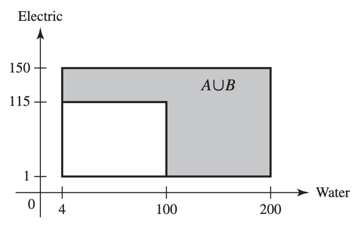
Figure 3.1:The event that at least one utility demand is high in Example 3.1.3.
The Distribution of a Random Variable
When a probability measure has been specified on the sample space of an experiment, we can determine probabilities associated with the possible values of each random variable . Let be a subset of the real line such that is an event, and let denote the probability that the value of will belong to the subset . Then is equal to the probability that the outcome of the experiment will be such that . In symbols,
It is a straightforward consequence of the definition of the distribution of that this distribution is itself a probability measure on the set of real numbers. The set will be an event for every set of real numbers that most readers will be able to imagine.
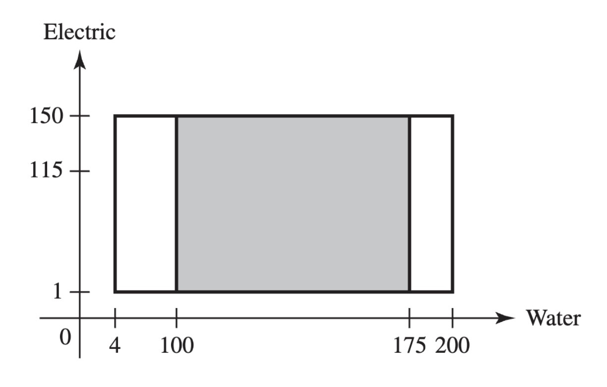
Figure 3.2:The event that water demand is between 50 and 175 in Example 3.1.5
The general definition of distribution in Definition 3.1.2 is awkward, and it will be useful to find alternative ways to specify the distributions of random variables. In the remainder of this section, we shall introduce a few such alternatives.
Discrete Distributions
Random variables that can take every value in an interval are said to have continuous distributions and are discussed in 3.2 Continuous Distributions.
Here are some simple facts about probability mass functions.
A typical pmf is sketched in Figure 3.3, in which each vertical segment represents the value of corresponding to a possible value . The sum of the heights of the vertical segments in Figure 3.3 must be 1.
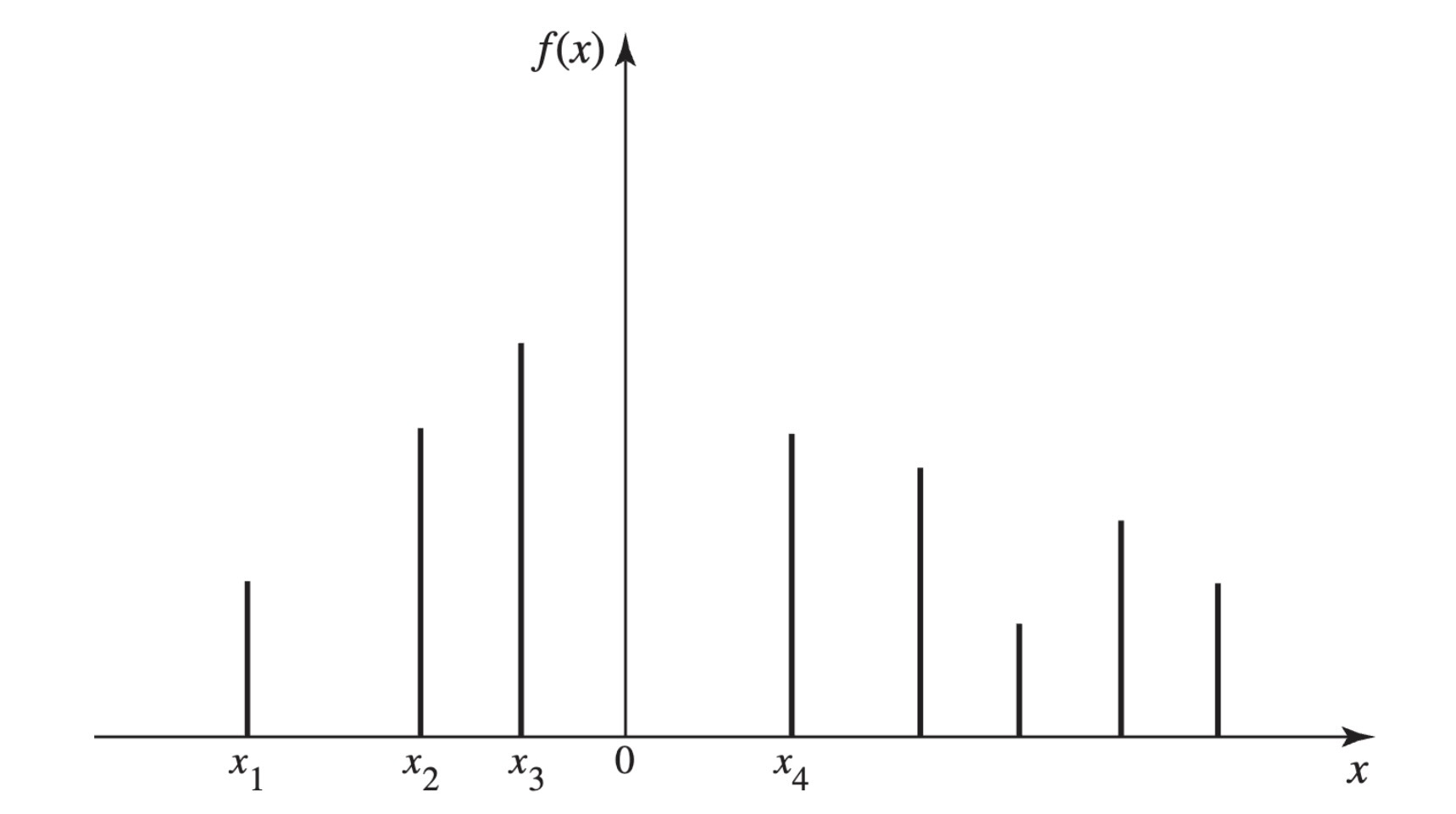
Figure 3.3:An example of a pmf
Theorem 3.1.2 shows that the pmf of a discrete random variable characterizes its distribution, and it allows us to dispense with the general definition of distribution when we are discussing discrete random variables.
Some random variables have distributions that appear so frequently that the distributions are given names. The random variable in Example 3.1.6 is one such example.
The in Example 3.1.6 has the Bernoulli distribution with parameter 0.65252. It is easy to see that the name of each Bernoulli distribution is enough to allow us to compute the pmf, which, in turn, allows us to characterize its distribution.
We conclude this section with illustrations of two additional families of discrete distributions that arise often enough to have names.
Uniform Distributions on Integers
The in Example 3.1.8 has the uniform distribution on the integers . A uniform distribution on a set of integers has probability on each integer. If , there are integers from to including and . The next result follows immediately from what we have just seen, and it illustrates how the name of the distribution characterizes the distribution.
The uniform distribution on the integers represents the outcome of an experiment that is often described by saying that one of the integers is chosen at random. In this context, the phrase “at random” means that each of the integers is equally likely to be chosen. In this same sense, it is not possible to choose an integer at random from the set of all positive integers, because it is not possible to assign the same probability to every one of the positive integers and still make the sum of these probabilities equal to 1. In other words, a uniform distribution cannot be assigned to an infinite sequence of possible values, but such a distribution can be assigned to any finite sequence.
Note: Random Variables Can Have the Same Distribution without Being the Same Random Variable. Consider two consecutive daily number draws as in Example 3.1.8. The sample space consists of all 6-tuples , where the first three coordinates are the numbers drawn on the first day and the last three are the numbers drawn on the second day (all in the order drawn). If , let and let . It is easy to see that and are different functions of and are not the same random variable. Indeed, there is only a small probability that they will take the same value. But they have the same distribution because they assume the same values with the same probabilities. If a businessman has 1000 customers numbered , and he selects one at random and records the number , the distribution of will be the same as the distribution of and of , but is not like or in any other way.
Binomial Distributions
Example 3.1.9: Defective Parts (p. 98)
Consider again exm-2-2-5. In that example, a machine produces a defective item with probability () and produces a nondefective item with probability . We assumed that the events that the different items were defective were mutually independent. Suppose that the experiment consists of examining of these items. Each outcome of this experiment will consist of a list of which items are defective and which are not, in the order examined. For example, we can let 0 stand for a nondefective item and 1 stand for a defective item. Then each outcome is a string of digits, each of which is 0 or 1. To be specific, if, say, , then some of the possible outcomes are
{#eq-3-1-3}
We will let denote the number of these items that are defective. Then the random variable will have a discrete distribution, and the possible values of will be . For example, the first four outcomes listed in eq-3-1-3 all have . The last outcome listed has .
Div is a generalization of exm-2-2-5 with items inspected rather than just six, and rewritten in the notation of random variables. For , the probability of obtaining each particular ordered sequence of items containing exactly defectives and nondefectives is , just as it was in exm-2-2-5. Since there are different ordered sequences of this type, it follows that
Therefore, the pmf of will be as follows:
{#eq-3-1-4}
Definition 3.1.7: Binomial Distribution/Random Variable
The discrete distribution represented by the pmf in eq-3-1-4 is called the binomial distribution with parameters and . A random variable with this distribution is said to be a binomial random variable with parameters and .
The reader should be able to verify that the random variable in Example 3.1.4, the number of heads in a sequence of 10 independent tosses of a fair coin, has the binomial distribution with parameters 10 and .
Since the name of each binomial distribution is sufficient to construct its pmf, it follows that the name is enough to identify the distribution. The name of each distribution includes the two parameters. The binomial distributions are very important in probability and statistics and will be discussed further in later chapters of this book.
A short table of values of certain binomial distributions is given at the end of this book. It can be found from this table, for example, that if has the binomial distribution with parameters and , then and .
As another example, suppose that a clinical trial is being run. Suppose that the probability that a patient recovers from her symptoms during the trial is and that the probability is that the patient does not recover. Let denote the number of patients who recover out of independent patients in the trial. Then the distribution of is also binomial with parameters and . Indeed, consider a general experiment that consists of observing independent repititions (trials) with only two possible results for each trial. For convenience, call the two possible results “success” and “failure.” Then the distribution of the number of trials that result in success will be binomial with parameters and , where is the probability of success on each trial.
Note: Names of Distributions. In this section, we gave names to several families of distributions. The name of each distribution includes any numerical parameters that are part of the definition. For example, the random variable in Example 3.1.4 has the binomial distribution with parameters 10 and . It is a correct statement to say that has a binomial distribution or that has a discrete distribution, but such statements are only partial descriptions of the distribution of . Such statements are not sufficient to name the distribution of , and hence they are not sufficient as answers to the question “What is the distribution of ?” The same considerations apply to all of the named distributions that we introduce elsewhere in the book. When attempting to specify the distribution of a random variable by giving its name, one must give the full name, including the values of any parameters. Only the full name is sufficient for determining the distribution.
Summary
A random variable is a real-valued function defined on a sample space. The distribution of a random variable is the collection of all probabilities for all subsets of the real numbers such that is an event. A random variable is discrete if there are at most countably many possible values for . In this case, the distribution of can be characterized by the probability mass function pmf of , namely, for in the set of possible values. Some distributions are so famous that they have names. One collection of such named distributions is the collection of uniform distributions on finite sets of integers. A more famous collection is the collection of binomial distributions whose parameters are and , where is a positive integer and , having pmf eq-3-1-4. The binomial distribution with parameters and is also called the Bernoulli distribution with parameter . The names of these distributions also characterize the distributions.
Exercises
Exercise 3.1.1
Suppose that a random variable has the uniform distribution on the integers . Find the probability that is even.
Exercise 3.1.2
Suppose that a random variable has a discrete distribution with the following pmf:
Determine the value of the constant .
Exercise 3.1.3
Suppose that two balanced dice are rolled, and let denote the absolute value of the difference between the two numbers that appear. Determine and sketch the pmf of .
Exercise 3.1.4
Suppose that a fair coin is tossed 10 times independently. Determine the pmf of the number of heads that will be obtained.
Exercise 3.1.5
Suppose that a box contains seven red balls and three blue balls. If five balls are selected at random, without replacement, determine the pmf of the number of red balls that will be obtained.
Exercise 3.1.6
Suppose that a random variable has the binomial distribution with parameters and . Find .
Exercise 3.1.7
Suppose that a random variable has the binomial distribution with parameters and . Find by using the table given at the end of this book. Hint: Use the fact that , where has the binomial distribution with parameters and .
Exercise 3.1.8
If 10 percent of the balls in a certain box are red, and if 20 balls are selected from the box at random, with replacement, what is the probability that more than three red balls will be obtained?
Exercise 3.1.9
Suppose that a random variable has a discrete distribution with the following pmf:
Find the value of the constant .
Exercise 3.1.10
A civil engineer is studying a left-turn lane that is long enough to hold seven cars. Let be the number of cars in the lane at the end of a randomly chosen red light. The engineer believes that the probability that is proportional to for (the possible values of ).
a. Find the pmf of . b. Find the probability that will be at least 5.
Exercise 3.1.11
Show that there does not exist any number such that the following function would be a pmf: