Overview
Next, we focus on random variables that can assume every value in an interval (bounded or unbounded). If a random variable has associated with it a function such that the integral of over each interval gives the probability that X is in the interval, then we call the probability density function (pdf) of and we say that has a continuous distribution.
The Probability Density Function
The water demand in Example 3.2.1 is an example of the following.
For example, in the situation described in Definition 3.2.1, for each bounded closed interval ,
Similarly, and .
We see that the function characterizes the distribution of a continuous random variable in much the same way that the probability mass function characterizes the distribution of a discrete random variable. For this reason, the function plays an important role, and hence we give it a name.
Example 3.2.1 demonstrates that the water demand has pdf given by (3.2.1).
Every pdf must satisfy the following two requirements:
and
A typical pdf is sketched in Figure 3.4. In that figure, the total area under the curve must be 1, and the value of is equal to the area of the shaded region.
Note: Continuous Distributions Assign Probability 0 to Individual Values. The integral in (3.2.3) also equals as well as and . Hence, it follows from the definition of continuous distributions that, if has a continuous distribution, for each number . As we noted on page 20, the fact that does not imply that is impossible. If it did, all values of would be impossible and couldn’t assume any value. What happens is that the probability in the distribution of is spread so thinly that we can only see it on sets like nondegenerate intervals. It is much the same as the fact that lines have 0 area in two dimensions, but that does not mean that lines are not there. The two vertical lines indicated under the curve in Figure 3.4 have 0 area, and this signifies that . However, for each and each such that , .
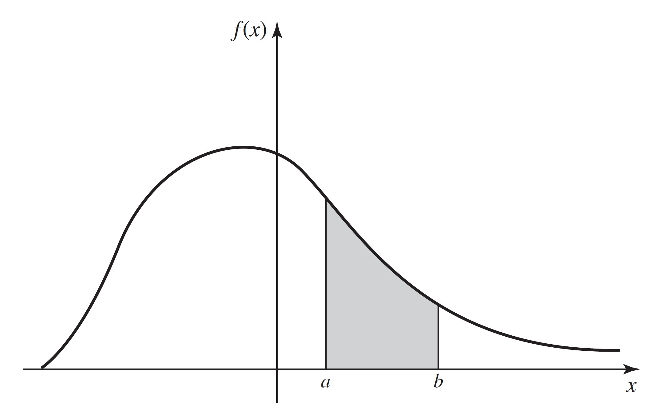
Figure 3.4:An example of a pdf
Nonuniqueness of the PDF
If a random variable has a continuous distribution, then for every individual value . Because of this property, the values of each pdf can be changed at a finite number of points, or even at certain infinite sequences of points, without changing the value of the integral of the pdf over any subset . In other words, the values of the pdf of a random variable can be changed arbitrarily at many points without affecting any probabilities involving , that is, without affecting the probability distribution of . At exactly which sets of points we can change a pdf depends on subtle features of the definition of the Riemann integral. We shall not deal with this issue in this text, and we shall only contemplate changes to pdfs at finitely many points.
To the extent just described, the pdf of a random variable is not unique. In many problems, however, there will be one version of the pdf that is more natural than any other because for this version the pdf will, wherever possible, be continuous on the real line. For example, the pdf sketched in Figure 3.4 is a continuous function over the entire real line. This pdf could be changed arbitrarily at a few points without affecting the probability distribution that it represents, but these changes would introduce discontinuities into the pdf without introducing any apparent advantages.
Throughout most of this book, we shall adopt the following practice: If a random variable has a continuous distribution, we shall give only one version of the pdf of and we shall refer to that version as the pdf of , just as though it had been uniquely determined. It should be remembered, however, that there is some freedom in the selection of the particular version of the pdf that is used to represent each continuous distribution. The most common place where such freedom will arise is in cases like (3.2.1) where the pdf is required to have discontinuities. Without making the function any less continuous, we could have defined the pdf in that example so that instead of . Both of these choices lead to the same calculations of all probabilities associated with , and they are both equally valid. Because the support of a continuous distribution is the closure of the set where the pdf is strictly positive, it can be shown that the support is unique. A sensible approach would then be to choose the version of the pdf that was strictly positive on the support whenever possible.
The reader should note that “continuous distribution” is not the name of a distribution, just as “discrete distribution” is not the name of a distribution. There are many distributions that are discrete and many that are continuous. Some distributions of each type have names that we either have introduced or will introduce later.
We shall now present several examples of continuous distributions and their PDFs.
Uniform Distributions on Intervals
Example 3.2.2: Temperature Forecasts
Television weather forecasters announce high and low temperature forecasts as integer numbers of degrees. These forecasts, however, are the results of very sophisticated weather models that provide more precise forecasts that the television personalities round to the nearest integer for simplicity. Suppose that the forecaster announces a high temperature of y. If we wanted to know what temperature the weather models actually produced, it might be safe to assume that was equally likely to be any number in the interval from to .
The distribution of in Div is a special case of the following.
Definition 3.2.3: Uniform Distribution on an Interval
Let and be two given real numbers such that . Let be a random variable such that it is known that and, for every subinterval of , the probability that will belong to that subinterval is proportional to the length of that subinterval. We then say that the random variable has the uniform distribution on the interval .
A random variable with the uniform distribution on the interval represents the outcome of an experiment that is often described by saying that a point is chosen at random from the interval . In this context, the phrase “at random” means that the point is just as likely to be chosen from any particular part of the interval as from any other part of the same length.
Theorem 3.2.1: Uniform Distribution PDF
If has the uniform distribution on an interval , then the pdf of is
{#eq-3-2-6}
must take a value in the interval . Hence, the pdf of must be 0 outside of . Furthermore, since any particular subinterval of having a given length is as likely to contain as is any other subinterval having the same length, regardless of the location of the particular subinterval in , it follows that must be constant throughout , and that interval is then the support of the distribution. Also,
{#eq-3-2-7}
Therefore, the constant value of throughout must be , and the pdf of must be eq-3-2-6.
![The pdf for the uniform distribution on the interval $[a, b]$.](ch03/images/fig-3-5.jpeg){#fig-3-5}

The pdf @eq-3-2-6 is sketched in @fig-3-5. As an example, the random variable $X$ (demand for water) in @exm-3-2-1 has the uniform distribution on the interval $[4, 200]$.

## Note: Density Is Not Probability

The reader should note that the pdf in @eq-3-2-6 can be greater than 1, particularly if $b − a < 1$. Indeed, pdfs can be unbounded, as we shall see in @exm-3-2-6. The pdf of $X$, $f(x)$, itself does not equal the probability that $X$ is near $x$. The integral of $f$ over values near $x$ gives the probability that $X$ is near $x$, and the integral is never greater than 1.

It is seen from @eq-3-2-6 that the pdf representing a uniform distribution on a given interval is constant over that interval, and the constant value of the pdf is the reciprocal of the length of the interval. It is not possible to define a uniform distribution over an unbounded interval, because the length of such an interval is infinite.

Consider again the uniform distribution on the interval $[a, b]$. Since the probability is 0 that one of the endpoints $a$ or $b$ will be chosen, it is irrelevant whether the distribution is regarded as a uniform distribution on the **closed** interval $a \leq x \leq b$, or as a uniform distribution on the **open** interval $a < x < b$, or as a uniform distribution on the half-open and half-closed interval $(a, b]$ in which one endpoint is included and the other endpoint is excluded.

For example, if a random variable $X$ has the uniform distribution on the interval $[−1, 4]$, then the pdf of $X$ is

$$
f(x) = \begin{cases}
1/5 &\text{for }-1 \leq x \leq 4, \\
0 &\text{otherwise.}
\end{cases}
$$

Furthermore,

$$
\Pr(0 \leq X < 2) = \int_{0}^{2}f(x)dx = \frac{2}{5}.
$$

Notice that we defined the pdf of $X$ to be strictly positive on the closed interval $[−1, 4]$ and 0 outside of this closed interval. It would have been just as sensible to define the pdf to be strictly positive on the open interval $(−1, 4)$ and 0 outside of this open interval. The probability distribution would be the same either way, including
the calculation of $\Pr(0 \leq X < 2)$ that we just performed. After this, when there are several equally sensible choices for how to define a pdf, we will simply choose one of them without making any note of the other choices.

(sec-3-2-4)
# Other Continuous Distributions

::: {#exm-3-2-3}

# Example 3.2.3: Incompletely Specified pdf

Suppose that the pdf of a certain random variable $X$ has the following form:

$$
f(x) = \begin{cases}
cx &\text{for }0 < x < 4, \\
0 &\text{otherwise,}
\end{cases}
$$

where $c$ is a given constant. We shall determine the value of $c$.

For every pdf, it must be true that $\int_{-\infty}^{\infty}f(x) = 1$. Therefore, in this example,

$$
\int_{0}^{4}cx~dx = 8c = 1.
$$

Hence, $c = 1/8$.
Note: Calculating Normalizing Constants. The calculation in exm-3-2-3 illustrates an important point that simplifies many statistical results. The pdf of was specified without explicitly giving the value of the constant . However, we were able to figure out what was the value of by using the fact that the integral of a pdf must be 1. It will often happen, especially in sec-8 where we find sampling distributions of summaries of observed data, that we can determine the pdf of a random variable except for a constant factor. That constant factor must be the unique value such that the integral of the pdf is 1, even if we cannot calculate it directly.
Example 3.2.4: Calculating Probabilities from a PDF (p. 105)
Suppose that the PDF of is as in exm-3-2-3, namely,
We shall now determine the values of and . Apply (3.2.3) to get
and
Example 3.2.5: Unbounded Random Variables
It is often convenient and useful to represent a continuous distribution by a pdf that is positive over an unbounded interval of the real line. For example, in a practical problem, the voltage in a certain electrical system might be a random variable with a continuous distribution that can be approximately represented by the pdf
{#eq-3-2-8}
It can be verified that the properties (3.2.4) and (3.2.5) required of all pdfs are satisfied by .
Even though the voltage may actually be bounded in the real situation, the pdf eq-3-2-8 may provide a good approximation for the distribution of over its full range of values. For example, suppose that it is known that the maximum possible value of is 1000, in which case . When the pdf eq-3-2-8 is used, we compute . If eq-3-2-8 adequately represents the variability of over the interval , then it may be more convenient to use the pdf eq-3-2-8 than a pdf that is similar to eq-3-2-8 for , except for a new normalizing constant, and is 0 for . This can be especially true if we do not know for sure that the maximum voltage is only 1000.
Example 3.2.6: Unbounded PDFs
Since a value of a PDF is a probability density, rather than a probability, such a value can be larger than 1. In fact, the values of the following PDF are unbounded in the neighborhood of :
{#eq-3-2-9}
It can be verified that even though the PDF eq-3-2-9 is unbounded, it satisfies the properties (3.2.4) and (3.2.5) required of a PDF.
Mixed Distributions
Most distributions that are encountered in practical problems are either discrete or continuous. We shall show, however, that it may sometimes be necessary to consider a distribution that is a mixture of a discrete distribution and a continuous distribution.
Example 3.2.7: Truncated Voltage (DeGroot and Schervish, p. 106)
Suppose that in the electrical system considered in Div, the voltage is to be measured by a voltmeter that will record the actual value of if but will simply record the value 3 if . If we let denote the value recorded by the voltmeter, then the distribution of can be derived as follows.
First, . Since the single value has probability , it follows that . Furthermore, since for , this probability for is distributed over the interval according to the same PDF (3.2.8) as that of over the same interval. Thus, the distribution of is specified by the combination of a PDF over the interval and a positive probability at the point .
Summary
A continuous distribution is characterized by its probability density function (PDF). A nonnegative function is the PDF of the distribution of if, for every interval , . Continuous random variables satisfy for every value . If the PDF of a distribution is constant on an interval and is 0 off the interval, we say that the distribution is uniform on the interval .
Exercises
Exercise 3.2.2
Suppose that the PDF of a random variable is as follows:
Sketch this PDF and determine the values of the following probabilities:
(a)
(b)
(c)
Exercise 3.2.3
Suppose that the PDF of a random variable is as follows:
Sketch this pdf and determine the values of the following probabilities:
(a)
(b)
(c) .
Exercise 3.2.4
Suppose that the pdf of a random variable is as follows:
a. Find the value of the constant and sketch the pdf. b. Find the value of .
Exercise 3.2.5
Suppose that the pdf of a random variable is as follows:
a. Find the value of such that . b. Find the value of such that .
Exercise 3.2.6
Let be a random variable for which the pdf is as given in Div. After the value of has been observed, let be the integer closest to . Find the pmf of the random variable .
Exercise 3.2.7
Suppose that a random variable has the uniform distribution on the interval . Find the pdf of and the value of .
Exercise 3.2.8
Suppose that the pdf of a random variable is as follows:
(a) Find the value of the constant and sketch the PDF.
(b) Find the value of .
Exercise 3.2.9
Show that there does not exist any number such that the following function would be a pdf:
Exercise 3.2.10
Suppose that the pdf of a random variable is as follows:
a. Find the value of the constant and sketch the pdf. b. Find the value of .
Exercise 3.2.11
Show that there does not exist any number such that the following function would be a pdf:
Exercise 3.2.12
In Example 3.1.3, determine the distribution of the random variable , the electricity demand. Also, find .
Exercise 3.2.13
An ice cream seller takes 20 gallons of ice cream in her truck each day. Let stand for the number of gallons that she sells. The probability is 0.1 that . If she doesn’t sell all 20 gallons, the distribution of follows a continuous distribution with a pdf of the form
where is a constant that makes . Find the constant so that as described above.