2 Conditional Probability

2.1 The Definition of Conditional Probability

A major use of probability in statistical inference is the updating of probabilities when certain events are observed. The updated probability of event $A$ after we learn that event $B$ has occurred is the conditional probability of $A$ given $B$.

Note

Example 2.1 (Example 2.1.1: Lottery Ticket) Consider a state lottery game in which six numbers are drawn without replacement from a bin containing the numbers 1–30. Each player tries to match the set of six numbers that will be drawn without regard to the order in which the numbers are drawn. Suppose that you hold a ticket in such a lottery with the numbers 1, 14, 15, 20, 23, and 27. You turn on your television to watch the drawing but all you see is one number, 15, being drawn when the power suddenly goes off in your house. You don’t even know whether 15 was the first, last, or some in-between draw. However, now that you know that 15 appears in the winning draw, the probability that your ticket is a winner must be higher than it was before you saw the draw. How do you calculate the revised probability?

Example 2.1 is typical of the following situation. An experiment is performed for which the sample space $S$ is given (or can be constructed easily) and the probabilities are available for all of the events of interest. We then learn that some event $B$ has occuured, and we want to know how the probability of another event $A$ changes after we learn that $B$ has occurred. In Example 2.1, the event that we have learned is $B = \{\text{one of the numbers drawn is }15\}$. We are certainly interested in the probability of

\[ A = \{\text{the numbers 1, 14, 15, 20, 23, and 27 are drawn}\}, \]

and possibly other events.

If we know that the event $B$ has occurred, then we know that the outcome of the experiment is one of those included in $B$. Hence, to evaluate the probability that $A$ will occur, we must consider the set of those outcomes in $B$ that also result in the occurrence of $A$. As sketched in Figure 2.1, this set is precisely the set $A \cap B$. It is therefore natural to calculate the revised probability of $A$ according to the following definition.

Figure 2.1: The outcomes in the event $B$ that also belong to the event $A$

Tip

Definition 2.1 (Definition 2.1.1: Conditional Probability) Suppose that we learn that an event $B$ has occurred and that we wish to compute the probability of another event $A$ taking into account that we know that $B$ has occurred. The new probability of $A$ is called the conditional probability of the event $A$ given that the event $B$ has occurred and is denoted $\Pr(A \mid B)$. If $\Pr(B) > 0$, we compute this probability as

\[ \Pr(A \mid B) = \frac{\Pr(A \cap B)}{\Pr(B)}. \tag{2.1}\]

The conditional probability $\Pr(A \mid B)$ is not defined if $\Pr(B) = 0$.

For convenience, the notation in Definition 2.1 is read simply as the conditional probability of $A$ given $B$. Equation 2.1 indicates that $\Pr(A \mid B)$ is computed as the proportion of the total probability $\Pr(B)$ that is represented by $\Pr(A \cap B)$, intuitively the proportion of $B$ that is also part of $A$.

Tip

Example 2.2 (Example 2.1.2: Lottery Ticket.) In Example 2.1, you learned that the event

\[ B = \{\text{one of the numbers drawn is }15\} \]

has occurred. You want to calculate the probability of the event $A$ that your ticket is a winner. Both events $A$ and $B$ are expressible in the sample space that consists of the $\binom{30}{6} = 30!/(6!24!)$ possible combinations of 30 items taken six at a time, namely, the unordered draws of six numbers from 1–30. The event $B$ consists of combinations that include 15. Since there are 29 remaining numbers from which to choose the other five in the winning draw, there are $\binom{29}{5}$ outcomes in $B$. It follows that

\[ \Pr(B) = \frac{\binom{29}{5}}{\binom{30}{6}} = \frac{29!24!6!}{30!5!24!} = 0.2. \]

The event $A$ that your ticket is a winner consists of a single outcome that is also in $B$, so $A \cap B = A$, and

\[ \Pr(A \cap B) = \Pr(A) = \frac{1}{\binom{30}{6}} = \frac{6!24!}{30!} = 1.68 \times 10^{-6}. \]

It follows that the conditional probability of $A$ given $B$ is

\[ \Pr(A \mid B) = \frac{\frac{6!24!}{30!}}{0.2} = 8.4 \times 10^{-6}. \]

This is five times as large as $\Pr(A)$ before you learned that $B$ had occurred.

Definition 2.1 for the conditional probability $\Pr(A \mid B)$ is worded in terms of the subjective interpretation of probability in Section 1.2. Equation 2.1 also has a simple meaning in terms of the frequency interpretation of probability. According to the frequency interpretation, if an experimental process is repeated a large number of times, then the proportion of repetitions in which the event $B$ will occur is approximately $\Pr(B)$ and the proportion of repetitions in which both the event $A$ and the event $B$ will occur is approximately $\Pr(A \cap B)$. Therefore, among those repetitions in which the event $B$ occurs, the proportion of repetitions in which the event $A$ will also occur is approximately equal to

\[ \Pr(A \mid B) = \frac{\Pr(A \cap B)}{\Pr(B)} \]

Tip

Example 2.3 (Example 2.1.3: Rolling Dice) Suppose that two dice were rolled and it was observed that the sum $T$ of the two numbers was odd. We shall determine the probability that $T$ was less than 8.

If we let $A$ be the event that $T < 8$ and let $B$ be the event that $T$ is odd, then $A \cap B$ is the event that $T$ is 3, 5, or 7. From the probabilities for two dice given at the end of Section 1.6, we can evaluate $\Pr(A \cap B)$ and $\Pr(B)$ as follows:

\[ \begin{align*} \Pr(A \cap B) &= \frac{2}{36} + \frac{4}{36} + \frac{6}{36} = \frac{12}{36} = \frac{1}{3}, \\ \Pr(B) &= \frac{2}{36} + \frac{4}{36} + \frac{6}{36} + \frac{4}{36} + \frac{2}{36} = \frac{18}{36} = \frac{1}{2}. \end{align*} \]

Hence,

\[ \Pr(A \mid B) = \frac{\Pr(A \cap B)}{\Pr(B)} = \frac{2}{3}. \]

Tip

Example 2.4 (Example 2.1.4: A Clinical Trial) It is very common for patients with episodes of depression to have a recurrence within two to three years. Prien et al. (1984) studied three treatments for depression: imipramine, lithium carbonate, and a combination. As is traditional in such studies (called clinical trials), there was also a group of patients who received a placebo. (A placebo is a treatment that is supposed to be neither helpful nor harmful. Some patients are given a placebo so that they will not know that they did not receive one of the other treatments. None of the other patients knew which treatment or placebo they received, either.) In this example, we shall consider 150 patients who entered the study after an episode of depression that was classified as “unipolar” (meaning that there was no manic disorder). They were divided into the four groups (three treatments plus placebo) and followed to see how many had recurrences of depression. ?tbl-2-1 summarizes the results. If a patient were selected at random from this study and it were found that the patient received the placebo treatment, what is the conditional probability that the patient had a relapse? Let $B$ be the event that the patient received the placebo, and let $A$ be the event that the patient had a relapse. We can calculate $\Pr(B) = 34/150$ and $\Pr(A \cap B) = 24/150$ directly from the table. Then $\Pr(A \mid B) = 24/34 = 0.706$. On the other hand, if the randomly selected patient is found to have received lithium (call this event $C$) then $\Pr(C) = 38/150$, $\Pr(A \cap C) = 13/150$, and $\Pr(A \mid C) = 13/38 = 0.342$. Knowing which treatment a patient received seems to make a difference to the probability of relapse. In Chapter 10, we shall study methods for being more precise about how much of a difference it makes.

Results of the clinical depression study in Example 2.4 {#tbl-2-1}
	Treatment Group
Response	Imipramine	Lithium	Combination	Placebo	Total
Relapse	18	13	22	24	77
No relapse	22	25	16	10	73
Total	40	38	38	34	150

Tip

Example 2.5 (Example 2.1.5: Rolling Dice Repeatedly) Suppose that two dice are to be rolled repeatedly and the sum $T$ of the two numbers is to be observed for each roll. We shall determine the probability $p$ that the value $T = 7$ will be observed before the value $T = 8$ is observed.

The desired probability $p$ could be calculated directly as follows: We could assume that the sample space $S$ contains all sequences of outcomes that terminate as soon as either the sum $T = 7$ or the sum $T = 8$ is obtained. Then we could find the sum of the probabilities of all the sequences that terminate when the value $T = 7$ is obtained.

However, there is a simpler approach in this example.We can consider the simple experiment in which two dice are rolled. If we repeat the experiment until either the sum $T = 7$ or the sum $T = 8$ is obtained, the effect is to restrict the outcome of the experiment to one of these two values. Hence, the problem can be restated as follows: Given that the outcome of the experiment is either $T = 7$ or $T = 8$, determine the probability $p$ that the outcome is actually $T = 7$.

If we let $A$ be the event that $T = 7$ and let $B$ be the event that the value of $T$ is either 7 or 8, then $A \cap B = A$ and

\[ p = \Pr(A \mid B) = \frac{\Pr(A \cap B)}{\Pr(B)} = \frac{\Pr(A)}{\Pr(B)}. \]

From the probabilities for two dice given in Example 1.14, $\Pr(A) = 6/36$ and $\Pr(B) = (6/36) + (5/36) = 11/36$. Hence, $p = 6/11$.

2.1.1 The Multiplication Rule for Conditional Probabilities

In some experiments, certain conditional probabilities are relatively easy to assign directly. In these experiments, it is then possible to compute the probability that both of two events occur by applying the next result that follows directly from Equation 2.1 and the analogous definition of $\Pr(B \mid A)$.

Tip

Theorem 2.1 (Theorem 2.1.1: Multiplication Rule for Conditional Probabilities) Let $A$ and $B$ be events. If $\Pr(B) > 0$, then

\[ \Pr(A \cap B) = \Pr(B)\Pr(A \mid B). \]

If $\Pr(A) > 0$, then

\[ \Pr(A \cap B) = \Pr(A)\Pr(B \mid A). \]

Tip

Example 2.6 (Example 2.1.6: Selecting Two Balls) Suppose that two balls are to be selected at random, without replacement, from a box containing $r$ red balls and $b$ blue balls. We shall determine the probability $p$ that the first ball will be red and the second ball will be blue.

Let $A$ be the event that the first ball is red, and let $B$ be the event that the second ball is blue. Obviously, $\Pr(A) = r/(r + b)$. Furthermore, if the event $A$ has occurred, then one red ball has been removed from the box on the first draw. Therefore, the probability of obtaining a blue ball on the second draw will be

\[ \Pr(B \mid A) = \frac{b}{r + b - 1}. \]

It follows that

\[ \Pr(A \cap B) = \frac{r}{r + b}\cdot \frac{b}{r + b - 1}. \]

The principle that has just been applied can be extended to any finite number of events, as stated in the following theorem.

Tip

Theorem 2.2 (Theorem 2.1.2: Multiplication Rule for Conditional Probabilities) Suppose that $A_1, A_2, \ldots, A_n$ are events such that $\Pr(A_1 \cap A_2 \cap \cdots \cap A_{n-1}) > 0$. Then

\[ \begin{align*} &\Pr(A_1 \cap A_2 \cap \cdots \cap A_n) \\ &=\Pr(A_1)\Pr(A_2 \mid A_1)\Pr(A_3 \mid A_1 \cap A_2)\cdots \Pr(A_n \mid A_1 \cap A_2 \cap \cdots \cap A_{n-1}). \end{align*} \tag{2.2}\]

Proof. The product of probabilities on the right side of Equation 2.2 is equal to

\[ \Pr(A_1)\cdot \frac{\Pr(A_1 \cap A_2)}{\Pr(A_1)} \cdot \frac{\Pr(A_1 \cap A_2 \cap A_3)}{\Pr(A_1 \cap A_2)}\cdots \frac{\Pr(A_1 \cap A_2 \cap \cdots \cap A_n)}{\Pr(A_1 \cap A_2 \cap \cdots \cap A_{n-1})}. \]

Since $\Pr(A_1 \cap A_2 \cap \cdots \cap A_{n-1}) > 0$, each of the denominators in this product must be positive. All of the terms in the product cancel each other except the final numerator $\Pr(A_1 \cap A_2 \cap \cdots \cap A_n)$, which is the left side of Equation 2.2.

Tip

Example 2.7 (Example 2.1.7: Selcting Four Balls) Suppose that four balls are selected one at a time, without replacement, from a box containing $r$ red balls and $b$ blue balls ($r \geq 2$, $b \geq 2$). We shall determine the probability of obtaining the sequence of outcomes red, blue, red, blue.

If we let $R_j$ denote the event that a red ball is obtained on the $j$th draw and let $B_j$ denote the event that a blue ball is obtained on the $j$th draw ($j = 1, \ldots, 4$), then

\[ \begin{align*} \Pr(R_1 \cap B_2 \cap R_3 \cap B_4) &= \Pr(R_1)\Pr(B_2 \mid R_1)\Pr(R_3 \mid R_1 \cap B_2)\Pr(B_4 \mid R_1 \cap B_2 \cap R_3) \\ &= \frac{r}{r+b} \cdot \frac{b}{r + b - 1} \cdot \frac{r-1}{r + b - 2} \cdot \frac{b - 1}{r + b - 3}. \end{align*} \]

Note: Conditional Probabilities Behave Just Like Probabilities. In all of the situations that we shall encounter in this text, every result that we can prove has a conditional version given an event $B$ with $\Pr(B) > 0$. Just replace all probabilities by conditional probabilities given $B$ and replace all conditional probabilities given other events $C$ by conditional probabilities given $C \cap B$. For example, Theorem 1.14 says that $\Pr(A^c) = 1 − \Pr(A)$. It is easy to prove that $\Pr(A^c \mid B) = 1 − \Pr(A \mid B)$ if $\Pr(B) > 0$. (See Exercises 2.11 and 2.12 in this section.) Another example is Theorem 2.3, which is a conditional version of the multiplication rule Theorem 2.2. Although a proof is given for Theorem 2.3, we shall not provide proofs of all such conditional theorems, because their proofs are generally very similar to the proofs of the unconditional versions.

Tip

Theorem 2.3 (Theorem 2.1.3) Suppose that $A_1, A_2, \ldots, A_n$, $B$ are events such that $\Pr(B) > 0$ and $\Pr(A_1 \cap A_2 \cap \cdots \cap A_{n-1} \mid B) > 0$. Then

\[ \begin{align*} \Pr(A_1 \cap A_2 \cap \cdots \cap A_n \mid B) = &\Pr(A_1 \mid B)\Pr(A_2 \mid A_1 \cap B)\cdots \\ &\cdot \Pr(A_n \mid A_1 \cap A_2 \cap \cdots \cap A_{n-1} \cap B). \end{align*} \tag{2.3}\]

Proof. The product of probabilities on the right side of Equation 2.3 is equal to

\[ \frac{\Pr(A_1 \cap B)}{\Pr(B)} \cdot \frac{\Pr(A_1 \cap A_2 \cap B)}{\Pr(A_1 \cap B)} \cdots \frac{\Pr(A_1 \cap A_2 \cap \cdots \cap A_n \cap B)}{\Pr(A_1 \cap A_2 \cap \cdots \cap A_{n-1} \cap B)}. \]

Since $\Pr(A_1 \cap A_2 \cap \cdots \cap A_{n-1} \mid B) > 0$, each of the denominators in this product must be positive. All of the terms in the product cancel each other except the first denominator and the final numerator to yield $\Pr(A_1 \cap A_2 \cap \cdots \cap A_n \cap B) / \Pr(B)$, which is the left side of Equation 2.3.

2.1.2 Conditional Probability and Partitions

Theorem 1.11 shows how to calculate the probability of an event by partitioning the sample space into two events $B$ and $B^c$. This result easily generalizes to larger partitions, and when combined with Theorem 2.1 it leads to a very powerful tool for calculating probabilities.

Tip

Definition 2.2 (Definition 2.1.2: Partition) Let $S$ denote the sample space of some experiment, and consider $k$ events $B_1, \ldots, B_k$ in $S$ such that $B_1, \ldots, B_k$ are disjoint and $\bigcup_{i=1}^kB_i = S$. It is said that these events form a partition of $S$.

Typically, the events that make up a partition are chosen so that an important source of uncertainty in the problem is reduced if we learn which event has occurred.

Tip

Example 2.8 (Example 2.1.8: Selecting Bolts) Two boxes contain long bolts and short bolts. Suppose that one box contains 60 long bolts and 40 short bolts, and that the other box contains 10 long bolts and 20 short bolts. Suppose also that one box is selected at random and a bolt is then selected at random from that box. We would like to determine the probability that this bolt is long.

Partitions can facilitate the calculations of probabilities of certain events.

Tip

Theorem 2.4 (Theorem 2.1.4: Law of Total Probability) Suppose that the events $B_1, \ldots, B_k$ form a partition of the space $S$ and $\Pr(B_j) > 0$ for $j = 1, \ldots, k$. Then, for every event $A$ in $S$,

\[ \Pr(A) = \sum_{j=1}^k \Pr(B_j)\Pr(A \mid B_j). \tag{2.4}\]

Proof. The events $B_1 \cap A, B_2 \cap A, \ldots, B_k \cap A$ will form a partition of $A$, as illustrated in Figure 2.2. Hence, we can write

\[ A = (B_1 \cap A) \cup (B_2 \cap A) \cup \cdots \cup (B_k \cap A). \]

Furthermore, since the $k$ events on the right side of this equation are disjoint,

\[ \Pr(A) = \sum_{j=1}^k \Pr(B_j \cap A). \]

Finally, if $\Pr(B_j) > 0$ for $j = 1, \ldots, k$, then $\Pr(B_j \cap A) = \Pr(B_j)\Pr(A \mid B_j)$ and it follows that Equation 2.4 holds.

Figure 2.2: The intersections of $A$ with events $B_1, \ldots, B_5$ of a partition in the proof of Theorem 2.4

Tip

Example 2.9 (Example 2.1.9: Selecting Bolts) In Example 2.8, let $B_1$ be the event that the first box (the one with 60 long and 40 short bolts) is selected, let $B_2$ be the event that the second box (the one with 10 long and 20 short bolts) is selected, and let $A$ be the event that a long bolt is selected. Then

\[ \Pr(A) = \Pr(B_1) \Pr(A \mid B_1) + \Pr(B_2) \Pr(A \mid B_2). \]

Since a box is selected at random, we know that $\Pr(B_1) = \Pr(B_2) = 1/2$. Furthermore, the probability of selecting a long bolt from the first box is $\Pr(A \mid B_1) = 60/100 = 3/5$, and the probability of selecting a long bolt from the second box is $\Pr(A \mid B_2) = 10/30 = 1/3$. Hence,

\[ \Pr(A) = \frac{1}{2}\cdot \frac{3}{5} + \frac{1}{2} \cdot \frac{1}{3} = \frac{7}{15}. \]

Tip

Example 2.10 (Example 2.1.10: Achieving a High Score) Suppose that a person plays a game in which his score must be one of the 50 numbers $1, 2, \ldots, 50$ and that each of these 50 numbers is equally likely to be his score. The first time he plays the game, his score is $X$. He then continues to play the game until he obtains another score $Y$ such that $Y \geq X$. We will assume that, conditional on previous plays, the 50 scores remain equally likely on all subsequent plays. We shall determine the probability of the event $A$ that $Y = 50$.

For each $i = 1, \ldots, 50$, let $B_i$ be the event that $X = i$. Conditional on $B_i$, the value of $Y$ is equally likely to be any one of the numbers $i, i + 1, \ldots, 50$. Since each of these $(51− i)$ possible values for $Y$ is equally likely, it follows that

\[ \Pr(A \mid B_i) = \Pr(Y = 50 \mid B_i) = \frac{1}{51-i}. \]

Furthermore, since the probability of each of the 50 values of $X$ is $1/50$, it follows that $\Pr(B_i) = 1/50$ for all $i$ and

\[ \Pr(A) = \sum_{i=1}^{50}\frac{1}{50}\cdot\frac{1}{51-i} = \frac{1}{50}\left(1 + \frac{1}{2} + \frac{1}{3} + \cdots + \frac{1}{50}\right) = 0.0900. \]

Note: Conditional Version of Law of Total Probability. The law of total probability has an analog conditional on another event $C$, namely,

\[ \Pr(A \mid C) = \sum_{j=1}^k \Pr(B_j \mid C)\Pr(A \mid B_j \cap C). \tag{2.5}\]

The reader can prove this in Exercise 2.17.

Augmented Experiment: In some experiments, it may not be clear from the initial description of the experiment that a partition exists that will facilitate the calculation of probabilities. However, there are many such experiments in which such a partition exists if we imagine that the experiment has some additional structure. Consider the following modification of Examples 2.8 and 2.9.

Tip

Example 2.11 (Example 2.1.11: Selecting Bolts) There is one box of bolts that contains some long and some short bolts. A manager is unable to open the box at present, so she asks her employees what is the composition of the box. One employee says that it contains 60 long bolts and 40 short bolts. Another says that it contains 10 long bolts and 20 short bolts. Unable to reconcile these opinions, the manager decides that each of the employees is correct with probability $1/2$. Let $B_1$ be the event that the box contains 60 long and 40 short bolts, and let $B_2$ be the event that the box contains 10 long and 20 short bolts. The probability that the first bolt selected is long is now calculated precisely as in Example 2.9.

In Example 2.11, there is only one box of bolts, but we believe that it has one of two possible compositions. We let the events $B_1$ and $B_2$ determine the possible compositions. This type of situation is very common in experiments.

Tip

Example 2.12 (Example 2.1.12: A Clinical Trial) Consider a clinical trial such as the study of treatments for depression in Example 2.4. As in many such trials, each patient has two possible outcomes, in this case relapse and no relapse. We shall refer to relapse as “failure” and no relapse as “success.” For now, we shall consider only patients in the imipramine treatment group. If we knew the effectiveness of imipramine, that is, the proportion $p$ of successes among all patients who might receive the treatment, then we might model the patients in our study as having probability $p$ of success. Unfortunately, we do not know $p$ at the start of the trial. In analogy to the box of bolts with unknown composition in Example 2.11, we can imagine that the collection of all available patients (from which the 40 imipramine patients in this trial were selected) has two or more possible compositions. We can imagine that the composition of the collection of patients determines the proportion that will be success. For simplicity, in this example, we imagine that there are 11 different possible compositions of the collection of patients. In particular, we assume that the proportions of success for the 11 possible compositions are $0, 1/10, \ldots, 9/10, 1$. (We shall be able to handle more realistic models for $p$ in Chapter 3.) For example, if we knew that our patients were drawn from a collection with the proportion $3/10$ of successes, we would be comfortable saying that the patients in our sample each have success probability $p = 3/10$. The value of $p$ is an important source of uncertainty in this problem, and we shall partition the sample space by the possible values of $p$. For $j = 1, \ldots, 11$, let $B_j$ be the event that our sample was drawn from a collection with proportion $(j − 1)/10$ of successes. We can also identify $B_j$ as the event $\{p = (j − 1)/10\}$.

Now, let $E_1$ be the event that the first patient in the imipramine group has a success. We defined each event $B_j$ so that $\Pr(E_1 \mid B_j) = (j − 1)/10$. Supppose that, prior to starting the trial, we believe that $\Pr(B_j) = 1/11$ for each $j$. It follows that

\[ \Pr(E_1) = \sum_{j=1}^{11}\frac{1}{11}\frac{j-1}{10} = \frac{55}{110} = \frac{1}{2}, \tag{2.6}\]

where the second equality uses the fact that $_{j=1}^n j = n(n+1)/2

The events $B_1, B_2, \ldots, B_{11}$ in Example 2.12 can be thought of in much the same way as the two events $B_1$ and $B_2$ that determine the mixture of long and short bolts in Example 2.11. There is only one box of bolts, but there is uncertainty about its composition. Similarly in Example 2.12, there is only one group of patients, but we believe that it has one of 11 possible compositions determined by the events $B_1, B_2, \ldots, B_{11}$. To call these events, they must be subsets of the sample space for the experiment in question. That will be the case in Example 2.12 if we imagine that the experiment consists not only of observing the numbers of successes and failures among the patients but also of potentially observing enough additional patients to be able to compute $p$, possibly at some time very far in the future. Similarly, in Example 2.11, the two events $B_1$ and $B_2$ are subsets of the sample space if we imagine that the experiment consists not only of observing one sample bolt but also of potentially observing the entire composition of the box.

Throughout the remainder of this text, we shall implicitly assume that experiments are augmented to include outcomes that determine the values of quantities such as $p$. We shall not require that we ever get to observe the complete outcome of the experiment so as to tell us precisely what $p$ is, but merely that there is an experiment that includes all of the events of interest to us, including those that determine quantities like $p$.

Tip

Definition 2.3 (Definition 2.1.3: Augmented Experiment) If desired, any experiment can be augmented to include the potential or hypothetical observation of as much additional information as we would find useful to help us calculate any probabilities that we desire.

Definition 2.3 is worded somewhat vaguely because it is intended to cover a wide variety of cases. Here is an explicit application to Example 2.12.

Tip

Example 2.13 (Example 2.1.13: A Clinical Trial) In Example 2.12, we could explicitly assume that there exists an infinite sequence of patients who could be treated with imipramine even though we will observe only finitely many of them. We could let the sample space consist of infinite sequences of the two symbols $S$ and $F$ such as $(S, S, F, S, F, F, F, \ldots)$. Here $S$ in coordinate $i$ means that the $i$th patient is a success, and $F$ stands for failure. So, the event $E_1$ in Example 2.12 is the event that the first coordinate is $S$. The example sequence above is then in the event $E_1$. To accommodate our interpretation of $p$ as the proportion of successes, we can assume that, for every such sequence, the proportion of $S$’s among the first $n$ coordinates gets close to one of the numbers $0, 1/10, \ldots, 9/10, 1$ as $n$ increases. In this way, $p$ is explicitly the limit of the proportion of successes we would observe if we could find a way to observe indefinitely. In Example 2.12, $B_2$ is the event consisting of all the outcomes in which the limit of the proportion of $S$’s equals $1/10$, $B_3$ is the set of outcomes in which the limit is $2/10$, etc. Also, we observe only the first 40 coordinates of the infinite sequence, but we still behave as if $p$ exists and could be determined if only we could observe forever.

In the remainder of the text, there will be many experiments that we assume are augmented. In such cases, we will mention which quantities (such as $p$ in Example 2.13) would be determined by the augmented part of the experiment even if we do not explicitly mention that the experiment is augmented.

2.1.3 The Game of Craps

We shall conclude this section by discussing a popular gambling game called craps. One version of this game is played as follows: A player rolls two dice, and the sum of the two numbers that appear is observed. If the sum on the first roll is 7 or 11, the player wins the game immediately. If the sum on the first roll is 2, 3, or 12, the player loses the game immediately. If the sum on the first roll is 4, 5, 6, 8, 9, or 10, then the two dice are rolled again and again until the sum is either 7 or the original value. If the original value is obtained a second time before 7 is obtained, then the player wins. If the sum 7 is obtained before the original value is obtained a second time, then the player loses.

We shall now compute the probability $\Pr(W)$, where $W$ is the event that the player will win. Let the sample space $S$ consist of all possible sequences of sums from the rolls of dice that might occur in a game. For example, some of the elements of $S$ are $(4, 7)$, $(11)$, $(4, 3, 4)$, $(12)$, $(10, 8, 2, 12, 6, 7)$, etc. We see that $(11) \in W$ but $(4, 7) \in W^c$, etc. We begin by noticing that whether or not an outcome is in $W$ depends in a crucial way on the first roll. For this reason, it makes sense to partition $W$ according to the sum on the first roll. Let $B_i$ be the event that the first roll is $i$ for $i = 2, \ldots, 12$.

Theorem 2.4 tells us that $\Pr(W) = \sum_{i=2}^{12}\Pr(B_i)\Pr(W \mid B_i)$. Since $\Pr(B_i)$ for each $i$ was computed in Example 1.14, we need to determine $\Pr(W \mid B_i)$ for each $i$. We begin with $i = 2$. Because the player loses if the first roll is 2, we have $\Pr(W \mid B_2) = 0$. Similarly, $\Pr(W \mid B_3) = 0 = \Pr(W \mid B_{12})$. Also, $\Pr(W \mid B_7) = 1$ because the player wins if the first roll is 7. Similarly, $\Pr(W \mid B_{11}) = 1$.

For each first roll $i \in \{4, 5, 6, 8, 9, 10\}$, $\Pr(W \mid B_i)$ is the probability that, in a sequence of dice rolls, the sum $i$ will be obtained before the sum 7 is obtained. As described in Example 2.5, this probability is the same as the probability of obtaining the sum $i$ when the sum must be either $i$ or 7. Hence,

\[ \Pr(W \mid B_i) = \frac{\Pr(B_i)}{\Pr(B_i \cup B_7)}. \]

We compute the necessary values here:

\[ \begin{align*} \Pr(W \mid B_4) &= \frac{\frac{3}{36}}{\frac{3}{36} + \frac{6}{36}} = \frac{1}{3}, \; \Pr(W \mid B_5) &= \frac{\frac{4}{36}}{\frac{4}{36} + \frac{6}{36}} = \frac{2}{5}, \\ \Pr(W \mid B_6) &= \frac{\frac{5}{36}}{\frac{5}{36} + \frac{6}{36}} = \frac{5}{11}, \; \Pr(W \mid B_8) &= \frac{\frac{5}{36}}{\frac{5}{36} + \frac{6}{36}} = \frac{5}{11}, \\ \Pr(W \mid B_9) &= \frac{\frac{4}{36}}{\frac{4}{36} + \frac{6}{36}} = \frac{2}{5}, \; \Pr(W \mid B_{10}) &= \frac{\frac{3}{36}}{\frac{3}{36} + \frac{6}{36}} = \frac{1}{3}. \end{align*} \]

Finally, we compute the sum $\sum_{i=2}^{12}\Pr(B_i)\Pr(W \mid B_i)$:

\[ \begin{align*} \Pr(W) &= \sum_{i=2}^{12}\Pr(B_i)\Pr(W \mid B_i) = 0 + 0 + \frac{3}{36}\frac{1}{3} + \frac{4}{36}\frac{2}{5} + \frac{5}{36}\frac{5}{11} + \frac{6}{36} \\ &+ \frac{5}{36}\frac{5}{11} + \frac{4}{36}\frac{2}{5} + \frac{3}{36}\frac{1}{3} + \frac{2}{36} + 0 = \frac{2928}{5940} = 0.493. \end{align*} \]

Thus, the probability of winning in the game of craps is slightly less than $1/2$.

2.1.4 Summary

The revised probability of an event $A$ after learning that event $B$ (with $\Pr(B) > 0$) has occurred is the conditional probability of $A$ given $B$, denoted by $\Pr(A \mid B)$ and computed as $\Pr(A \cap B) / \Pr(B)$. Often it is easy to assess a conditional probability, such as $\Pr(A \mid B)$, directly. In such a case, we can use the multiplication rule for conditional probabilities to compute $\Pr(A \cap B) = \Pr(B)\Pr(A \mid B)$. All probability results have versions conditional on an event $B$ with $\Pr(B) > 0$: Just change all probabilities so that they are conditional on $B$ in addition to anything else they were already conditional on. For example, the multiplication rule for conditional probabilities becomes $\Pr(A_1 \cap A_2 \mid B) = \Pr(A_1 \mid B)\Pr(A_2 \mid A_1 \cap B)$. A partition is a collection of disjoint events whose union is the whole sample space. To be most useful, a partition is chosen so that an important source of uncertainty is reduced if we learn which one of the partition events occurs. If the conditional probability of an event $A$ is available given each event in a partition, the law of total probability tells how to combine these conditional probabilities to get $\Pr(A)$.

2.1.5 Exercises

Exercise 2.1 (Exercise 2.1.1) If $A \subset B$ with $\Pr(B) > 0$, what is the value of $\Pr(A \mid B)$?

Exercise 2.2 (Exercise 2.1.2) If $A$ and $B$ are disjoint events and $\Pr(B) > 0$, what is the value of $\Pr(A \mid B)$?

Exercise 2.3 (Exercise 2.1.3) If $S$ is the sample space of an experiment and $A$ is any event in that space, what is the value of $\Pr(A \mid S)$?

Exercise 2.4 (Exercise 2.1.4) Each time a shopper purchases a tube of toothpaste, he chooses either brand $A$ or brand $B$. Suppose that for each purchase after the first, the probability is $1/3$ that he will choose the same brand that he chose on his preceding purchase and the probability is $2/3$ that he will switch brands. If he is equally likely to choose either brand $A$ or brand $B$ on his first purchase, what is the probability that both his first and second purchases will be brand $A$ and both his third and fourth purchases will be brand $B$?

Exercise 2.5 (Exercise 2.1.5) A box contains $r$ red balls and $b$ blue balls. One ball is selected at random and its color is observed. The ball is then returned to the box and $k$ additional balls of the same color are also put into the box. A second ball is then selected at random, its color is observed, and it is returned to the box together with $k$ additional balls of the same color. Each time another ball is selected, the process is repeated. If four balls are selected, what is the probability that the first three balls will be red and the fourth ball will be blue?

Exercise 2.6 (Exercise 2.1.6) A box contains three cards. One card is red on both sides, one card is green on both sides, and one card is red on one side and green on the other. One card is selected from the box at random, and the color on one side is observed. If this side is green, what is the probability that the other side of the card is also green?

Exercise 2.7 (Exercise 2.1.7) Consider again the conditions of Exercise 1.83 of Section 1.10. If a family selected at random from the city subscribes to newspaper $A$, what is the probability that the family also subscribes to newspaper $B$?

Exercise 2.8 (Exercise 2.1.8) Consider again the conditions of Exercise 1.83 of Section 1.10. If a family selected at random from the city subscribes to at least one of the three newspapers $A$, $B$, and $C$, what is the probability that the family subscribes to newspaper $A$?

Exercise 2.9 (Exercise 2.1.9) Suppose that a box contains one blue card and four red cards, which are labeled $A$, $B$, $C$, and $D$. Suppose also that two of these five cards are selected at random, without replacement.

If it is known that card $A$ has been selected, what is the probability that both cards are red?
If it is known that at least one red card has been selected, what is the probability that both cards are red?

Exercise 2.10 (Exercise 2.1.10) Consider the following version of the game of craps: The player rolls two dice. If the sum on the first roll is 7 or 11, the player wins the game immediately. If the sum on the first roll is 2, 3, or 12, the player loses the game immediately. However, if the sum on the first roll is 4, 5, 6, 8, 9, or 10, then the two dice are rolled again and again until the sum is either 7 or 11 or the original value. If the original value is obtained a second time before either 7 or 11 is obtained, then the player wins. If either 7 or 11 is obtained before the original value is obtained a second time, then the player loses. Determine the probability that the player will win this game.

Exercise 2.11 (Exercise 2.1.11) For any two events $A$ and $B$ with $\Pr(B) > 0$, prove that $\Pr(A^c \mid B) = 1 − \Pr(A \mid B)$.

Exercise 2.12 (Exercise 2.1.12) For any three events $A$, $B$, and $D$, such that $\Pr(D) > 0$, prove that $\Pr(A \cup B \mid D) = \Pr(A \mid D) + \Pr(B \mid D) − \Pr(A \cap B \mid D)$.

Exercise 2.13 (Exercise 2.1.13) A box contains three coins with a head on each side, four coins with a tail on each side, and two fair coins. If one of these nine coins is selected at random and tossed once, what is the probability that a head will be obtained?

Exercise 2.14 (Exercise 2.1.14) A machine produces defective parts with three different probabilities depending on its state of repair. If the machine is in good working order, it produces defective parts with probability 0.02. If it is wearing down, it produces defective parts with probability 0.1. If it needs maintenance, it produces defective parts with probability 0.3. The probability that the machine is in good working order is 0.8, the probability that it is wearing down is 0.1, and the probability that it needs maintenance is 0.1. Compute the probability that a randomly selected part will be defective.

Exercise 2.15 (Exercise 2.1.15) The percentages of voters classed as Liberals in three different election districts are divided as follows: in the first district, 21 percent; in the second district, 45 percent; and in the third district, 75 percent. If a district is selected at random and a voter is selected at random from that district, what is the probability that she will be a Liberal?

Exercise 2.16 (Exercise 2.1.16) Consider again the shopper described in Exercise 2.4. On each purchase, the probability that he will choose the same brand of toothpaste that he chose on his preceding purchase is $1/3$, and the probability that he will switch brands is $2/3$. Suppose that on his first purchase the probability that he will choose brand $A$ is $1/4$ and the probability that he will choose brand $B$ is $3/4$. What is the probability that his second purchase will be brand $B$?

Exercise 2.17 (Exercise 2.1.17) Prove the conditional version of the law of total probability (Equation 2.5).

2.2 Independent Events

If learning that $B$ has occurred does not change the probability of $A$, then we say that $A$ and $B$ are independent. There are many cases in which events $A$ and $B$ are not independent, but they would be independent if we learned that some other event $C$ had occurred. In this case, $A$ and $B$ are conditionally independent given $C$.

Tip

Example 2.14 (Example 2.2.1: Tossing Coins) Suppose that a fair coin is tossed twice. The experiment has four outcomes, $HH$, $HT$, $TH$, and $TT$, that tell us how the coin landed on each of the two tosses. We can assume that this sample space is simple so that each outcome has probability $1/4$. Suppose that we are interested in the second toss. In particular, we want to calculate the probability of the event $A = \{H\text{ on second toss}\}$. We see that $A = \{HH, TH\}$, so that $\Pr(A) = 2/4 = 1/2$. If we learn that the first coin landed $T$, we might wish to compute the conditional probability $\Pr(A \mid B)$ where $B = \{T\text{ on first toss}\}$. Using the definition of conditional probability, we easily compute

\[ \Pr(A \mid B) = \frac{\Pr(A \cap B)}{\Pr(B)} = \frac{1/4}{1/2} = \frac{1}{2}, \]

because $A \cap B = \{TH\}$ has probability $1/4$. We see that $\Pr(A \mid B) = \Pr(A)$; hence, we don’t change the probability of $A$ even after we learn that $B$ has occurred.

2.2.1 Definition of Independence

The conditional probability of the event $A$ given that the event $B$ has occurred is the revised probability of $A$ after we learn that $B$ has occurred. It might be the case, however, that no revision is necessary to the probability of $A$ even after we learn that $B$ occurs. This is precisely what happened in Example 2.14. In this case, we say that $A$ and $B$ are independent events. As another example, if we toss a coin and then roll a die, we could let $A$ be the event that the die shows 3 and let $B$ be the event that the coin lands with heads up. If the tossing of the coin is done in isolation of the rolling of the die, we might be quite comfortable assigning $\Pr(A \mid B) = \Pr(A) = 1/6$. In this case, we say that $A$ and $B$ are independent events.

In general, if $\Pr(B) > 0$, the equation $\Pr(A \mid B) = \Pr(A)$ can be rewritten as $\Pr(A \cap B) / \Pr(B) = \Pr(A)$. If we multiply both sides of this last equation by $\Pr(B)$, we obtain the equation $\Pr(A \cap B) = \Pr(A)\Pr(B)$. In order to avoid the condition $\Pr(B) > 0$, the mathematical definition of the independence of two events is stated as follows:

Note

Definition 2.4 (Definition 2.2.1: Independent Events) Two events $A$ and $B$ are independent if

\[ \Pr(A \cap B) = \Pr(A)\Pr(B). \]

Suppose that $\Pr(A) > 0$ and $\Pr(B) > 0$. Then it follows easily from the definitions of independence and conditional probability that $A$ and $B$ are independent if and only if $\Pr(A \mid B) = \Pr(A)$ and $\Pr(B \mid A) = \Pr(B)$.

2.2.2 Independence of Two Events

If two events $A$ and $B$ are considered to be independent because the events are physically unrelated, and if the probabilities $\Pr(A)$ and $\Pr(B)$ are known, then the definition can be used to assign a value to $\Pr(A \cap B)$.

Tip

Example 2.15 (Example 2.2.2: Machine Operation) Suppose that two machines 1 and 2 in a factory are operated independently of each other. Let $A$ be the event that machine 1 will become inoperative during a given 8-hour period, let $B$ be the event that machine 2 will become inoperative during the same period, and suppose that $\Pr(A) = 1/3$ and $\Pr(B) = 1/4$. We shall determine the probability that at least one of the machines will become inoperative during the given period.

The probability $\Pr(A \cap B)$ that both machines will become inoperative during the period is

\[ \Pr(A \cap B) = \Pr(A)\Pr(B) = \left(\frac{1}{3}\right)\left(\frac{1}{4}\right) = \frac{1}{12}. \]

Therefore, the probability $\Pr(A \cup B)$ that at least one of the machines will become inoperative during the period is

\[ \begin{align*} \Pr(A \cup B) &= \Pr(A) + \Pr(B) − \Pr(A \cap B) \\ &= \frac{1}{3} + \frac{1}{4} - \frac{1}{12} = \frac{1}{2}. \end{align*} \]

The next example shows that two events $A$ and $B$, which are physically related, can, nevertheless, satisfy the definition of independence.

Tip

Example 2.16 (Example 2.2.3: Rolling a Die) Suppose that a balanced die is rolled. Let $A$ be the event that an even number is obtained, and let $B$ be the event that one of the numbers 1, 2, 3, or 4 is obtained. We shall show that the events $A$ and $B$ are independent.

In this example, $\Pr(A) = 1/2$ and $\Pr(B) = 2/3$. Furthermore, since $A \cap B$ is the event that either the number 2 or the number 4 is obtained, $\Pr(A \cap B) = 1/3$. Hence, $\Pr(A \cap B) = \Pr(A)\Pr(B)$. It follows that the events $A$ and $B$ are independent events, even though the occurrence of each event depends on the same roll of a die.

The independence of the events $A$ and $B$ in Example 2.16 can also be interpreted as follows: Suppose that a person must bet on whether the number obtained on the die will be even or odd, that is, on whether or not the event $A$ will occur. Since three of the possible outcomes of the roll are even and the other three are odd, the person will typically have no preference between betting on an even number and betting on an odd number.

Suppose also that after the die has been rolled, but before the person has learned the outcome and before she has decided whether to bet on an even outcome or on an odd outcome, she is informed that the actual outcome was one of the numbers 1, 2, 3, or 4, i.e., that the event $B$ has occurred. The person now knows that the outcome was 1, 2, 3, or 4. However, since two of these numbers are even and two are odd, the person will typically still have no preference between betting on an even number and betting on an odd number. In other words, the information that the event $B$ has occurred is of no help to the person who is trying to decide whether or not the event $A$ has occurred.

Independence of Complements: In the foregoing discussion of independent events, we stated that if $A$ and $B$ are independent, then the occurrence or nonoccurrence of $A$ should not be related to the occurrence or nonoccurrence of $B$. Hence, if $A$ and $B$ satisfy the mathematical definition of independent events, then it should also be true that $A$ and $B^c$ are independent events, that $A^c$ and $B$ are independent events, and that $A^c$ and $B^c$ are independent events. One of these results is established in the next theorem.

Theorem 2.5 (Theorem 2.2.1) If two events $A$ and $B$ are independent, then the events $A$ and $B^c$ are also independent.

Proof. Theorem 1.17 says that

\[ \Pr(A \cap B^c) = \Pr(A) − \Pr(A \cap B). \]

Furthermore, since $A$ and $B$ are independent events, $\Pr(A \cap B) = \Pr(A)\Pr(B)$. It now follows that

\[ \begin{align*} \Pr(A \cap B^c) &= \Pr(A) − \Pr(A)\Pr(B) = \Pr(A)[1 − \Pr(B)] \\ &= \Pr(A)\Pr(B^c). \end{align*} \]

Therefore, the events $A$ and $B^c$ are independent.

The proof of the analogous result for the events $A^c$ and $B$ is similar, and the proof for the events $A^c$ and $B^c$ is required in Exercise 2.19 at the end of this section.

2.2.3 Independence of Several Events

The definition of independent events can be extended to any number of events, $A_1, \ldots, A_k$. Intuitively, if learning that some of these events do or do not occur does not change our probabilities for any events that depend only on the remaining events, we would say that all $k$ events are independent. The mathematical definition is the following analog to Definition 2.4.

Tip

Definition 2.5 (Definition 2.2.2: (Mutually) Independent Events) The $k$ events $A_1, \ldots, A_k$ are independent (or mutually independent) if, for every subset $A_{i_1}, \ldots, A_{i_j}$ of $j$ of these events ($j = 2, 3, \ldots, k$),

\[ \Pr(A_{i_1} \cap \cdots \cap A_{i_j}) = \Pr(A_{i_1}) \cdots \Pr(A_{i_j}). \]

As an example, in order for three events $A$, $B$, and $C$ to be independent, the following four relations must be satisfied:

\[ \begin{align*} \Pr(A \cap B) = \Pr(A)\Pr(B), \\ \Pr(A \cap C) = \Pr(A)\Pr(C), \\ \Pr(B \cap C) = \Pr(B)\Pr(C), \end{align*} \tag{2.7}\]

and

\[ \Pr(A \cap B \cap C) = \Pr(A)\Pr(B)\Pr(C). \tag{2.8}\]

It is possible that Equation 2.8 will be satisfied, but one or more of the three relations Equation 2.7 will not be satisfied. On the other hand, as is shown in the next example, it is also possible that each of the three relations Equation 2.7 will be satisfied but Equation 2.8 will not be satisfied.

Tip

Example 2.17 (Example 2.2.4: Pairwise Independence) Suppose that a fair coin is tossed twice so that the sample space $S = \{HH, HT, TH, TT\}$ is simple. Define the following three events:

\[ \begin{align*} A &= \{H\text{ on first toss}\} = \{HH, HT\}, \\ B &= \{H\text{ on second toss}\} = \{HH, TH\},\text{ and} \\ C &= \{\text{Both tosses the same}\} = \{HH, TT\}. \end{align*} \]

Then $A \cap B = A \cap C = B \cap C = A \cap B \cap C = \{HH\}$. Hence,

\[ \Pr(A) = \Pr(B) = \Pr(C) = 1/2 \]

and

\[ \Pr(A \cap B) = \Pr(A \cap C) = \Pr(B \cap C) = \Pr(A \cap B \cap C) = 1/4. \]

It follows that each of the three relations of Equation 2.7 is satisfied but Equation 2.8 is not satisfied. These results can be summarized by saying that the events $A$, $B$, and $C$ are pairwise independent, but all three events are not independent.

We shall now present some examples that will illustrate the power and scope of the concept of independence in the solution of probability problems.

Tip

Example 2.18 (Example 2.2.5: Inspecting Items) Suppose that a machine produces a defective item with probability $p$ ($0 < p < 1$) and produces a nondefective item with probability $1 − p$. Suppose further that six items produced by the machine are selected at random and inspected, and that the results (defective or nondefective) for these six items are independent. We shall determine the probability that exactly two of the six items are defective.

It can be assumed that the sample space $S$ contains all possible arrangements of six items, each one of which might be either defective or nondefective. For $j = 1, \ldots, 6$, we shall let $D_j$ denote the event that the $j$th item in the sample is defective so that $D_j^c$ is the event that this item is nondefective. Since the outcomes for the six different items are independent, the probability of obtaining any particular sequence of defective and nondefective items will simply be the product of the individual probabilities for the items. For example,

\[ \begin{align*} \Pr(D_1^c \cap D_2 \cap D_3^c \cap D_4^c \cap D_5 \cap D_6^c) &= \Pr(D_1^c)\Pr(D_2)\Pr(D_3^c)\Pr(D_4^c)\Pr(D_5)\Pr(D_6^c) \\ &= (1-p)p(1-p)(1-p)p(1-p) = p^2(1-p)^4. \end{align*} \]

It can be seen that the probability of any other particular sequence in $S$ containing two defective items and four nondefective items will also be $p^2(1− p)^4$. Hence, the probability that there will be exactly two defectives in the sample of six items can be found by multiplying the probability $p^2(1− p)^4$ of any particular sequence containing two defectives by the possible number of such sequences. Since there are $\binom{6}{2}$ distinct arrangements of two defective items and four nondefective items, the probability of obtaining exactly two defectives is $\binom{6}{2}p^2(1-p)^4$.

Tip

Example 2.19 (Example 2.2.6: Obtaining a Defective Item) For the conditions of Example 2.18, we shall now determine the probability that at least one of the six items in the sample will be defective.

Since the outcomes for the different items are independent, the probability that all six items will be nondefective is $(1−p)^6$. Therefore, the probability that at least one item will be defective is $1 − (1 − p)^6$.

Tip

Example 2.20 (Example 2.2.7: Tossing a Coin Until a Head Appears) Suppose that a fair coin is tossed until a head appears for the first time, and assume that the outcomes of the tosses are independent. We shall determine the probability $p_n$ that exactly $n$ tosses will be required.

The desired probability is equal to the probability of obtaining $n − 1$ tails in succession and then obtaining a head on the next toss. Since the outcomes of the tosses are independent, the probability of this particular sequence of $n$ outcomes is $p_n = (1/2)^n$.

The probability that a head will be obtained sooner or later (or, equivalently, that tails will not be obtained forever) is

\[ \sum_{n=1}^{\infty}p_n = \frac{1}{2} + \frac{1}{4} + \frac{1}{8} + \cdots = 1. \]

Since the sum of the probabilities $p_n$ is 1, it follows that the probability of obtaining an infinite sequence of tails without ever obtaining a head must be 0.

Tip

Example 2.21 (Example 2.2.8: Inspecting Items One at a Time) Consider again a machine that produces a defective item with probability $p$ and produces a nondefective item with probability $1 − p$. Suppose that items produced by the machine are selected at random and inspected one at a time until exactly five defective items have been obtained. We shall determine the probability $p_n$ that exactly $n$ items ($n \geq 5$) must be selected to obtain the five defectives.

The fifth defective item will be the $n$th item that is inspected if and only if there are exactly four defectives among the first $n − 1$ items and then the $n$th item is defective. By reasoning similar to that given in Example 2.18, it can be shown that the probability of obtaining exactly four defectives and $n − 5$ nondefectives among the first $n − 1$ items is $\binom{n-1}{4}p^4(1-p)^{n-5}$. The probability that the $n$th item will be defective is $p$. Since the first event refers to outcomes for only the first $n − 1$ items and the second event refers to the outcome for only the $n$th item, these two events are independent. Therefore, the probability that both events will occur is equal to the product of their probabilities. It follows that

\[ p_n = \binom{n-1}{4}p^5(1-p)^{n-5} \]

Tip

Example 2.22 (Example 2.2.9: People v. Collins.) Finkelstein and Levin (1990) describe a criminal case whose verdict was overturned by the Supreme Court of California in part due to a probability calculation involving both conditional probability and independence. The case, People v. Collins, 68 Cal. 2d 319, 438 P.2d 33 (1968), involved a purse snatching in which witnesses claimed to see a young woman with blond hair in a ponytail fleeing from the scene in a yellow car driven by a black man with a beard. A couple meeting the description was arrested a few days after the crime, but no physical evidence was found. A mathematician calculated the probability that a randomly selected couple would possess the described characteristics as about $8.3 \times 10^{−8}$, or 1 in 12 million. Faced with such overwhelming odds and no physical evidence, the jury decided that the defendants must have been the only such couple and convicted them. The Supreme Court thought that a more useful probability should have been calculated. Based on the testimony of the witnesses, there was a couple that met the above description. Given that there was already one couple who met the description, what is the conditional probability that there was also a second couple such as the defendants?

Let $p$ be the probability that a randomly selected couple from a population of $n$ couples has certain characteristics. Let $A$ be the event that at least one couple in the population has the characteristics, and let $B$ be the event that at least two couples have the characteristics. What we seek is $\Pr(B \mid A)$. Since $B \subset A$, it follows that

\[ \Pr(B \mid A) = \frac{B \cap A}{\Pr(A)} = \frac{\Pr(B)}{\Pr(A)}. \]

We shall calculate $\Pr(B)$ and $\Pr(A)$ by breaking each event into more manageable pieces. Suppose that we number the $n$ couples in the population from 1 to $n$. Let $A_i$ be the event that couple number $i$ has the characteristics in question for $i = 1, \ldots, n$, and let $C$ be the event that exactly one couple has the characteristics. Then

\[ \begin{align*} A &= (A_1^c \cap A_2^c \cap \cdots \cap A_n^c)^c, \\ C &= (A_1 \cap A_2^c \cap \cdots \cap A_n^c) \cup (A_1^c \cap A_2 \cap A_3^c \cap \cdots \cap A_n^c) \cup \cdots \cup (A_1^c \cap \cdots \cap A_{n-1}^c \cap A_n), \\ B &= A \cap C^c. \end{align*} \]

Assuming that the $n$ couples are mutually independent, $\Pr(A^c) = (1 − p)^n$, and $\Pr(A) = 1− (1 − p)^n$. The $n$ events whose union is $C$ are disjoint and each one has probability $p(1− p)^{n−1}$, so $\Pr(C) = np(1 − p)^{n−1}$. Since $A = B \cup C$ with $B$ and $C$ disjoint, we have

\[ \Pr(B) = \Pr(A) − \Pr(C) = 1− (1 − p)^n − np(1− p)^{n−1}. \]

So,

\[ \Pr(B \mid A) = \frac{1 - (1-p)^n - np(1-p)^{n-1}}{1 - (1-p)^n}. \tag{2.9}\]

The Supreme Court of California reasoned that, since the crime occurred in a heavily populated area, $n$ would be in the millions. For example, with $p = 8.3 \times 10^{−8}$ and $n = 8,000,000$, the value of Equation 2.9 is 0.2966. Such a probability suggests that there is a reasonable chance that there was another couple meeting the same description as the witnesses provided. Of course, the court did not know how large $n$ was, but the fact that Equation 2.9 could easily be so large was grounds enough to rule that reasonable doubt remained as to the guilt of the defendants.

Independence and Conditional Probability: Two events $A$ and $B$ with positive probability are independent if and only if $\Pr(A \mid B) = \Pr(A)$. Similar results hold for larger collections of independent events. The following theorem, for example, is straightforward to prove based on the definition of independence.

Caution

Theorem 2.6 (Theorem 2.2.2) Let $A_1, \ldots, A_k$ be events such that $\Pr(A_1 \cap \cdots \cap A_k) > 0$. Then $A_1, \ldots, A_k$ are independent if and only if, for every two disjoint subsets $\{i_1, \ldots, i_m\}$ and $\{j_1, \ldots, j_\ell\}$ of $\{1, \ldots, k\}$, we have

\[ \Pr(A_{i_1} \cap \cdots \cap A_{i_m} \mid A_{j_1} \cap \cdots \cap A_{j_\ell}) = \Pr(A_{i_1} \cap \cdots \cap A_{i_m}). \]

Theorem 2.6 says that $k$ events are independent if and only if learning that some of the events occur does not change the probability that any combination of the other events occurs.

The Meaning of Independence: We have given a mathematical definition of independent events in Definition 2.4. We have also given some interpretations for what it means for events to be independent. The most instructive interpretation is the one based on conditional probability. If learning that $B$ occurs does not change the probability of $A$, then $A$ and $B$ are independent. In simple examples such as tossing what we believe to be a fair coin, we would generally not expect to change our minds about what is likely to happen on later flips after we observe earlier flips; hence, we declare the events that concern different flips to be independent. However, consider a situation similar to Example 2.18 in which items produced by a machine are inspected to see whether or not they are defective. In Example 2.18, we declared that the different items were independent and that each item had probability $p$ of being defective. This might make sense if we were confident that we knew how well the machine was performing. But if we were unsure of how the machine were performing, we could easily imagine changing our mind about the probability that the 10th item is defective depending on how many of the first nine items are defective. To be specific, suppose that we begin by thinking that the probability is 0.08 that an item will be defective. If we observe one or zero defective items in the first nine, we might not make much revision to the probability that the 10th item is defective. On the other hand, if we observe eight or nine defectives in the first nine items, we might be uncomfortable keeping the probability at 0.08 that the 10th item will be defective. In summary, when deciding whether to model events as independent, try to answer the following question: “If I were to learn that some of these events occurred, would I change the probabilities of any of the others?” If we feel that we already know everything that we could learn from these events about how likely the others should be, we can safely model them as independent. If, on the other hand, we feel that learning some of these events could change our minds about how likely some of the others are, then we should be more careful about determining the conditional probabilities and not model the events as independent.

Mutually Exclusive Events and Mutually Independent Events: Two similar-sounding definitions have appeared earlier in this text. Definition 1.11 defines mutually exclusive events, and Definition 2.5 defines mutually independent events. It is almost never the case that the same set of events satisfies both definitions. The reason is that if events are disjoint (mutually exclusive), then learning that one occurs means that the others definitely did not occur. Hence, learning that one occurs would change the probabilities for all the others to 0, unless the others already had probability 0. Indeed, this suggests the only condition in which the two definitions would both apply to the same collection of events. The proof of the following result is left to Exercise 2.41 in this section.

Caution

Theorem 2.7 (Theorem 2.2.3) Let $n > 1$ and let $A_1, \ldots, A_n$ be events that are mutually exclusive. The events are also mutually independent if and only if all the events except possibly one of them has probability 0.

2.2.4 Conditionally Independent Events

Conditional probability and independence combine into one of the most versatile models of data collection. The idea is that, in many circumstances, we are unwilling to say that certain events are independent because we believe that learning some of them will provide information about how likely the others are to occur. But if we knew the frequency with which such events would occur, we might then be willing to assume that they are independent. This model can be illustrated using one of the examples from earlier in this section.

Example 2.23 (Example 2.2.10: Inspecting Items) Consider again the situation in Example 2.18. This time, however, suppose that we believe that we would change our minds about the probabilities of later items being defective were we to learn that certain numbers of early items were defective. Suppose that we think of the number $p$ from Example 2.18 as the proportion of defective items that we would expect to see if we were to inspect a very large sample of items. If we knew this proportion $p$, and if we were to sample only a few, say, six or 10 items now, we might feel confident maintaining that the probability of a later item being defective remains $p$ even after we inspect some of the earlier items. On the other hand, if we are not sure what would be the proportion of defective items in a large sample, we might not feel confident keeping the probability the same as we continue to inspect.

To be precise, suppose that we treat the proportion $p$ of defective items as unknown and that we are dealing with an augmented experiment as described in Definition 2.3. For simplicity, suppose that $p$ can take one of two values, either 0.01 or 0.4, the first corresponding to normal operation and the second corresponding to a need for maintenance. Let $B_1$ be the event that $p = 0.01$, and let $B_2$ be the event that $p = 0.4$. If we knew that $B_1$ had occurred, then we would proceed under the assumption that the events $D_1, D_2, \ldots$ were independent with $\Pr(D_i \mid B_1) = 0.01$ for all $i$. For example, we could do the same calculations as in Examples 2.18 and 2.21 with $p = 0.01$. Let $A$ be the event that we observe exactly two defectives in a random sample of six items. Then $\Pr(A \mid B_1) = \binom{6}{2}(0.01)^2(0.99)^4 = 1.44 \times 10^{-3}$. Similarly, if we knew that $B_2$ had occurred, then we would assume that $D_1, D_2, \ldots$ were independent with $\Pr(D_i \mid B_2) = 0.4$. In this case, $\Pr(A \mid B_2) = \binom{6}{2}(0.4)^2(0.6)^4 = 0.311$.

In Example 2.23, there is no reason that $p$ must be required to assume at most two different values. We could easily allow $p$ to take a third value or a fourth value, etc. Indeed, in Chapter 3 we shall learn how to handle the case in which every number between 0 and 1 is a possible value of $p$. The point of the simple example is to illustrate the concept of assuming that events are independent conditional on another event, such as $B_1$ or $B_2$ in the example.

The formal concept illustrated in Example 2.23 is the following:

Note

Definition 2.6 (Definition 2.2.3: Conditional Independence) We say that events $A_1, \ldots, A_k$ are conditionally independent given $B$ if, for every subcollection $A_{i_1}, \ldots, A_{i_j}$ of $j$ of these events ($j = 2, 3, \ldots, k$),

\[ \Pr\left( A_{i_1} \cap \cdots \cap A_{i_j} \mid B \right) = \Pr(A_{i_1} \mid B)\cdots \Pr(A_{i_j} \mid B). \]

Definition 2.6 is identical to Definition 2.5 for independent events with the modification that all probabilities in the definition are now conditional on $B$. As a note, even if we assume that events $A_1, \ldots, A_k$ are conditionally independent given $B$, it is not necessary that they be conditionally independent given $B^c$. In Example 2.23, the events $D_1, D_2, \ldots$ were conditionally independent given both $B_1$ and $B_2 = B_1^c$, which is the typical situation. Exercise 2.57 in Section 2.3 is an example in which events are conditionally independent given one event $B$ but are not conditionally independent given the complement $B^c$.

Recall that two events $A_1$ and $A_2$ (with $\Pr(A_1) > 0$) are independent if and only if $\Pr(A_2 \mid A_1) = \Pr(A_2)$. A similar result holds for conditionally independent events.

Caution

Theorem 2.8 (Theorem 2.2.4) Suppose that $A_1$, $A_2$, and $B$ are events such that $\Pr(A_1 \cap B) > 0$. Then $A_1$ and $A_2$ are conditionally independent given $B$ if and only if $\Pr(A_2 \mid A_1 \cap B) = \Pr(A_2 \mid B)$.

This is another example of the claim we made earlier that every result we can prove has an analog conditional on an event $B$. The reader can prove this theorem in Exercise 2.39.

2.2.5 The Collector’s Problem

Suppose that $n$ balls are thrown in a random manner into $r$ boxes ($r \leq n$). We shall assume that the $n$ throws are independent and that each of the $r$ boxes is equally likely to receive any given ball. The problem is to determine the probability $p$ that every box will receive at least one ball. This problem can be reformulated in terms of a collector’s problem as follows: Suppose that each package of bubble gum contains the picture of a baseball player, that the pictures of $r$ different players are used, that the picture of each player is equally likely to be placed in any given package of gum, and that pictures are placed in different packages independently of each other. The problem now is to determine the probability $p$ that a person who buys $n$ packages of gum ($n \geq r$) will obtain a complete set of $r$ different pictures.

For $i = 1, \ldots, r$, let $A_i$ denote the event that the picture of player $i$ is missing from all $n$ packages. Then $\bigcup_{i=1}^r A_i$ is the event that the picture of at least one player is missing. We shall find $(_{i=1}^r A_i) by applying Equation 1.10.

Since the picture of each of the $r$ players is equally likely to be placed in any particular package, the probability that the picture of player $i$ will not be obtained in any particular package is $(r − 1)/r$. Since the packages are filled independently, the probability that the picture of player $i$ will not be obtained in any of the $n$ packages is $[(r − 1)/r]n$. Hence,

\[ \Pr(A_i) = \left(\frac{r-1}{r}\right)^n \; \text{ for }i = 1, \ldots, r. \]

Now consider any two players $i$ and $j$. The probability that neither the picture of player $i$ nor the picture of player $j$ will be obtained in any particular package is $(r − 2)/r$. Therefore, the probability that neither picture will be obtained in any of the $n$ packages is $[(r − 2)/r]n$. Thus,

\[ \Pr(A_i \cap A_j) = \left(\frac{r-2}{r}\right)^n. \]

If we next consider any three players $i$, $j$, and $k$, we find that

\[ \Pr(A_i \cap A_j \cap A_k) = \left(\frac{r - 3}{r}\right)^3. \]

By continuing in this way, we finally arrive at the probability $\Pr(A_1 \cap A_2 \cap \cdots \cap A_r)$ that the pictures of all $r$ players are missing from the $n$ packages. Of course, this probability is 0. Therefore, by Equation 1.10 of Section 1.10,

\[ \begin{align*} \Pr\left( \bigcup_{i=1}^r A_i \right) &= r \left(\frac{r-1}{r}\right)^n - \binom{r}{2}\left(\frac{r-2}{r}\right)^n + \cdots + (-1)^r\binom{r}{r-1}\left(\frac{1}{r}\right)^n \\ &= \sum_{j=1}^{r-1}(-1)^{j+1}\binom{r}{j}\left(1 - \frac{j}{r}\right)^n. \end{align*} \]

Since the probability $p$ of obtaining a complete set of $r$ different pictures is equal to $1 - \Pr(\bigcup_{i=1}^r A_i)$, it follows from the foregoing derivation that $p$ can be written in the form

\[ p = \sum_{j=0}^{r-1}(-1)^j \binom{r}{j}\left(1 - \frac{j}{r}\right)^n. \]

::: :::

2.2.6 Summary

A collection of events is independent if and only if learning that some of them occur does not change the probabilities that any combination of the rest of them occurs. Equivalently, a collection of events is independent if and only if the probability of the intersection of every subcollection is the product of the individual probabilities. The concept of independence has a version conditional on another event. A collection of events is independent conditional on $B$ if and only if the conditional probability of the intersection of every subcollection given $B$ is the product of the individual conditional probabilities given $B$. Equivalently, a collection of events is conditionally independent given $B$ if and only if learning that some of them (and $B$) occur does not change the conditional probabilities given $B$ that any combination of the rest of them occur. The full power of conditional independence will become more apparent after we introduce Bayes’ theorem in the next section.

2.2.7 Exercises

Exercise 2.18 (Exercise 2.2.1) If $A$ and $B$ are independent events and $\Pr(B) < 1$, what is the value of $\Pr(A^c \mid B^c)$?

Exercise 2.19 (Exercise 2.2.2) Assuming that $A$ and $B$ are independent events, prove that the events $A^c$ and $B^c$ are also independent.

Exercise 2.20 (Exercise 2.2.3) Suppose that $A$ is an event such that $\Pr(A) = 0$ and that $B$ is any other event. Prove that $A$ and $B$ are independent events.

Exercise 2.21 (Exercise 2.2.4) Suppose that a person rolls two balanced dice three times in succession. Determine the probability that on each of the three rolls, the sum of the two numbers that appear will be 7.

Exercise 2.22 (Exercise 2.2.5) Suppose that the probability that the control system used in a spaceship will malfunction on a given flight is 0.001. Suppose further that a duplicate, but completely independent, control system is also installed in the spaceship to take control in case the first system malfunctions. Determine the probability that the spaceship will be under the control of either the original system or the duplicate system on a given flight.

Exercise 2.23 (Exercise 2.2.6) Suppose that 10,000 tickets are sold in one lottery and 5000 tickets are sold in another lottery. If a person owns 100 tickets in each lottery, what is the probability that she will win at least one first prize?

Exercise 2.24 (Exercise 2.2.7) Two students $A$ and $B$ are both registered for a certain course. Assume that student $A$ attends class 80 percent of the time, student $B$ attends class 60 percent of the time, and the absences of the two students are independent.

What is the probability that at least one of the two students will be in class on a given day?
If at least one of the two students is in class on a given day, what is the probability that $A$ is in class that day?

Exercise 2.25 (Exercise 2.2.8) If three balanced dice are rolled, what is the probability that all three numbers will be the same?

Exercise 2.26 (Exercise 2.2.9) Consider an experiment in which a fair coin is tossed until a head is obtained for the first time. If this experiment is performed three times, what is the probability that exactly the same number of tosses will be required for each of the three performances?

Exercise 2.27 (Exercise 2.2.10) The probability that any child in a certain family will have blue eyes is $1/4$, and this feature is inherited independently by different children in the family. If there are five children in the family and it is known that at least one of these children has blue eyes, what is the probability that at least three of the children have blue eyes?

Exercise 2.28 (Exercise 2.2.11) Consider the family with five children described in Exercise 2.27.

If it is known that the youngest child in the family has blue eyes, what is the probability that at least three of the children have blue eyes?
Explain why the answer in part (a) is different from the answer in Exercise 2.27.

Exercise 2.29 (Exercise 2.2.12) Suppose that $A$, $B$, and $C$ are three independent events such that $\Pr(A) = 1/4$, $\Pr(B) = 1/3$, and $\Pr(C) = 1/2$.

Determine the probability that none of these three events will occur.
Determine the probability that exactly one of these three events will occur.

Exercise 2.30 (Exercise 2.2.13) Suppose that the probability that any particle emitted by a radioactive material will penetrate a certain shield is 0.01. If 10 particles are emitted, what is the probability that exactly one of the particles will penetrate the shield?

Exercise 2.31 (Exercise 2.2.14) Consider again the conditions of Exercise 2.30. If 10 particles are emitted, what is the probability that at least one of the particles will penetrate the shield?

Exercise 2.32 (Exercise 2.2.15) Consider again the conditions of Exercise 2.30. How many particles must be emitted in order for the probability to be at least 0.8 that at least one particle will penetrate the shield?

Exercise 2.33 (Exercise 2.2.16) In the World Series of baseball, two teams $A$ and $B$ play a sequence of games against each other, and the first team that wins a total of four games becomes the winner of the World Series. If the probability that team $A$ will win any particular game against team $B$ is $1/3$, what is the probability that team $A$ will win the World Series?

Exercise 2.34 (Exercise 2.2.17) Two boys $A$ and $B$ throw a ball at a target. Suppose that the probability that boy $A$ will hit the target on any throw is $1/3$ and the probability that boy $B$ will hit the target on any throw is $1/4$. Suppose also that boy $A$ throws first and the two boys take turns throwing. Determine the probability that the target will be hit for the first time on the third throw of boy $A$.

Exercise 2.35 (Exercise 2.2.18) For the conditions of Exercise 2.34, determine the probability that boy $A$ will hit the target before boy $B$ does.

Exercise 2.36 (Exercise 2.2.19) A box contains 20 red balls, 30 white balls, and 50 blue balls. Suppose that 10 balls are selected at random one at a time, with replacement; that is, each selected ball is replaced in the box before the next selection is made. Determine the probability that at least one color will be missing from the 10 selected balls.

Exercise 2.37 (Exercise 2.2.20) Suppose that $A_1, \ldots, A_k$ form a sequence of $k$ independent events. Let $B_1, \ldots, B_k$ be another sequence of $k$ events such that for each value of $j$ ($j = 1, \ldots, k$), either $B_j = A_j$ or $B_j = A_j^c$. Prove that $B_1, \ldots, B_k$ are also independent events. Hint: Use an induction argument based on the number of events $B_j$ for which $B_j = A_j^c$.

Exercise 2.38 (Exercise 2.2.21) Prove Theorem 2.6. Hint: The “only if” direction is direct from Definition 2.5. For the “if” direction, use induction on the value of $j$ in the definition of independence. Let $m = j − 1$ and let $\ell = 1$ with $j_1 = i_j$.

Exercise 2.39 (Exercise 2.2.22) Prove Theorem 2.8.

Exercise 2.40 (Exercise 2.2.23) A programmer is about to attempt to compile a series of 11 similar programs. Let $A_i$ be the event that the $i$th program compiles successfully for $i = 1, \ldots, 11$. When the programming task is easy, the programmer expects that 80 percent of programs should compile. When the programming task is difficult, she expects that only 40 percent of the programs will compile. Let $B$ be the event that the programming task was easy. The programmer believes that the events $A_1, \ldots, A_{11}$ are conditionally independent given $B$ and given $B^c$.

Compute the probability that exactly 8 out of 11 programs will compile given $B$.
Compute the probability that exactly 8 out of 11 programs will compile given $B^c$.

Exercise 2.41 (Exercise 2.2.24) Prove Theorem 2.7.

2.3 Bayes’ Theorem

Suppose that we are interested in which of several disjoint events $B_1, \ldots, B_k$ will occur and that we will get to observe some other event $A$. If $\Pr(A \mid B_i)$ is available for each $i$, then Bayes’ theorem is a useful formula for computing the conditional of the $B_i$ events given $A$.

We begin with a typical example.

Example 2.24 (Example 2.3.1: Test for a Disease) Suppose that you are walking down the street and notice that the Department of Public Health is giving a free medical test for a certain disease. The test is 90 percent reliable in the following sense: If a person has the disease, there is a probability of 0.9 that the test will give a positive response; whereas, if a person does not have the disease, there is a probability of only 0.1 that the test will give a positive response.

Data indicate that your chances of having the disease are only 1 in 10,000. However, since the test costs you nothing, and is fast and harmless, you decide to stop and take the test. A few days later you learn that you had a positive response to the test. Now, what is the probability that you have the disease?

The last question in Example 2.24 is a prototype of the question for which Bayes’ theorem was designed.We have at least two disjoint events (“you have the disease” and “you do not have the disease”) about which we are uncertain, and we learn a piece of information (the result of the test) that tells us something about the uncertain events. Then we need to know how to revise the probabilities of the events in the light of the information we learned.

We now present the general structure in which Bayes’ theorem operates before returning to the example.

2.3.1 Statement, Proof, and Examples of Bayes’ Theorem

Example 2.25 (Example 2.3.2: Selecting Bolts) Consider again the situation in Example 2.8, in which a bolt is selected at random from one of two boxes. Suppose that we cannot tell without making a further effort from which of the two boxes the one bolt is being selected. For example, the boxes may be identical in appearance or somebody else may actually select the box, but we only get to see the bolt. prior to selecting the bolt, it was equally likely that each of the two boxes would be selected. However, if we learn that event $A$ has occurred, that is, a long bolt was selected, we can compute the conditional of the two boxes given $A$. To remind the reader, $B_1$ is the event that the box is selected containing 60 long bolts and 40 short bolts, while $B_2$ is the event that the box is selected containing 10 long bolts and 20 short bolts. In Example 2.9, we computed $\Pr(A) = 7/15$, $\Pr(A \mid B_1) = 3/5$, $\Pr(A \mid B_2) = 1/3$, and $\Pr(B_1) = \Pr(B_2) = 1/2$. So, for example,

\[ \Pr(B_1 \mid A) = \frac{\Pr(A \cap B_1)}{\Pr(A)} = \frac{\Pr(B_1)\Pr(A \mid B_1)}{\Pr(A)} = \frac{\frac{1}{2}\cdot \frac{3}{5}}{\frac{7}{15}} = \frac{9}{14}. \]

Since the first box has a higher of long bolts than the second box, it seems reasonable that the probability of $B_1$ should rise after we learn that a long bolt was selected. It must be that $\Pr(B_2 \mid A) = 5/14$ since one or the other box had to be selected.

In Example 2.25, we started with uncertainty about which of two boxes would be chosen and then we observed a long bolt drawn from the chosen box. Because the two boxes have different chances of having a long bolt drawn, the observation of a long bolt changed the of each of the two boxes having been chosen. The calculation of how the change is the purpose of Bayes’ theorem.

Theorem 2.9 (Theorem 2.3.1: Bayes’ Theorem) Let the events $B_1, \ldots, B_k$ form a partition of the space $S$ such that $\Pr(B_j) > 0$ for $j = 1, \ldots, k$, and let $A$ be an event such that $\Pr(A) > 0$. Then, for $i = 1, \ldots, k$,

\[ \Pr(B_i \mid A) = \frac{\Pr(B_i)\Pr(A \mid B_i)}{\sum_{j=1}^k \Pr(B_j)\Pr(A \mid B_j)}. \tag{2.10}\]

Proof. By the definition of conditional probability,

\[ \Pr(B_i \mid A) = \frac{\Pr(B_i \cap A)}{\Pr(A)}. \]

The numerator on the right side of Equation 2.10 is equal to $\Pr(B_i \cap A)$ by Theorem 2.1. The denominator is equal to $\Pr(A)$ according to Theorem 2.4.

Example 2.26 (Example 2.3.3: Test for a Disease) Let us return to the example with which we began this section. We have just received word that we have tested positive for a disease. The test was 90 percent reliable in the sense that we described in Example 2.24. We want to know the probability that we have the disease after we learn that the result of the test is positive. Some readers may feel that this probability should be about 0.9. However, this feeling completely ignores the small probability of 0.0001 that you had the disease before taking the test. We shall let $B_1$ denote the event that you have the disease, and let $B_2$ denote the event that you do not have the disease. The events $B_1$ and $B_2$ form a partition. Also, let $A$ denote the event that the response to the test is positive. The event $A$ is information we will learn that tells us something about the partition elements. Then, by Bayes’ theorem,

\[ \begin{align*} \Pr(B_1 \mid A) &= \frac{\Pr(A \mid B_1)\Pr(B_1)}{\Pr(A \mid B_1)\Pr(B_1) + \Pr(A \mid B_2)\Pr(B_2)} \\ &= \frac{(0.9)(0.0001)}{(0.9)(0.0001) + (0.1)(0.9999)} = 0.00090. \end{align*} \]

Thus, the conditional probability that you have the disease given the test result is approximately only 1 in 1000. Of course, this conditional probability is approximately 9 times as great as the probability was before you were tested, but even the conditional probability is quite small.

Another way to explain this result is as follows: Only one person in every 10,000 actually has the disease, but the test gives a positive response for approximately one person in every 10. Hence, the number of positive responses is approximately 1000 times the number of persons who actually have the disease. In other words, out of every 1000 persons for whom the test gives a positive response, only one person actually has the disease. This example illustrates not only the use of Bayes’ theorem but also the importance of taking into account all of the information available in a .

Example 2.27 (Example 2.3.4: Identifying the Source of a Defective Item) Three different machines $M_1$, $M_2$, and $M_3$ were used for a large batch of similar manufactured items. Suppose that 20 percent of the items were by machine $M_1$, 30 percent by machine $M_2$, and 50 percent by machine $M_3$. Suppose further that 1 percent of the items by machine $M_1$ are defective, that 2 percent of the items by machine $M_2$ are defective, and that 3 percent of the items by machine $M_3$ are defective. Finally, suppose that one item is selected at random from the entire batch and it is found to be defective. We shall determine the probability that this item was by machine $M_2$.

Let $B_i$ be the event that the selected item was by machine $M_i$ ($i = 1, 2, 3$), and let $A$ be the event that the selected item is defective. We must evaluate the conditional probability $\Pr(B_2 \mid A)$.

The probability $\Pr(B_i)$ that an item selected at random from the entire batch was by machine $M_i$ is as follows, for $i = 1, 2, 3$:

\[ \Pr(B_1) = 0.2, \; \Pr(B_2) = 0.3, \; \Pr(B_3) = 0.5. \]

Furthermore, the probability $\Pr(A \mid B_i)$ that an item by machine $M_i$ will be defective is

\[ \Pr(A \mid B_1) = 0.01, \; \Pr(A \mid B_2) = 0.02, \Pr(A \mid B_3) = 0.03. \]

It now follows from Bayes’ theorem that

\[ \begin{align*} \Pr(B_2 \mid A) &= \frac{\Pr(B_2)\Pr(A \mid B_2)}{\sum_{j=1}^3 \Pr(B_j)\Pr(A \mid B_j)} \\ &= \frac{(0.3)(0.02)}{(0.2)(0.01) + (0.3)(0.02) + (0.5)(0.03)} = 0.26. \end{align*} \]

Example 2.28 (Example 2.3.5: Identifying Genotypes) Consider a gene that has two alleles (see Example 1.13) $A$ and $a$. Suppose that the gene exhibits itself through a trait (such as hair color or blood type) with two versions. We call $A$ dominant and $a$ recessive if individuals with genotypes $AA$ and $Aa$ have the same version of the trait and the individuals with genotype $aa$ have the other version. The two versions of the trait are called phenotypes. We shall call the phenotype exhibited by individuals with genotypes $AA$ and $Aa$ the dominant trait, and the other trait will be called the recessive trait. In population genetics studies, it is common to have information on the phenotypes of individuals, but it is rather difficult to determine genotypes. However, some information about genotypes can be obtained by observing phenotypes of parents and children.

Assume that the allele $A$ is dominant, that individuals mate independently of genotype, and that the genotypes $AA$, $Aa$, and $aa$ occur in the population with probabilities $1/4$, $1/2$, and $1/4$, respectively. We are going to observe an individual whose parents are not available, and we shall observe the phenotype of this individual. Let $E$ be the event that the observed individual has the dominant trait. We would like to revise our opinion of the possible genotypes of the parents. There are six possible genotype combinations, $B_1, \ldots, B_6$, for the parents prior to making any observations, and these are listed in Table 2.1.

The probabilities of the $B_i$ were computed using the assumption that the parents mated independently of genotype. For example, $B_3$ occurs if the father is $AA$ and the mother is $aa$ (probability $1/16$) or if the father is $aa$ and the mother is $AA$ (probability $1/16$). The values of $\Pr(E \mid B_i)$ were computed assuming that the two available alleles are passed from parents to children with probability $1/2$ each and independently for the two parents. For example, given $B_4$, the event $E$ occurs if and only if the child does not get two $a$’s. The probability of getting $a$ from both parents given $B_4$ is $1/4$, so $\Pr(E \mid B_4) = 3/4$.

Now we shall compute $\Pr(B_1 \mid E)$ and $\Pr(B_5 \mid E)$. We leave the other calculations to the reader. The denominator of Bayes’ theorem is the same for both calculations, namely,

\[ \begin{align*} \Pr(E) &= \sum_{i=1}^{5} \Pr(B_i)\Pr(E \mid B_i) \\ &= \frac{1}{16} \cdot 1 + \frac{1}{4} \cdot 1 + \frac{1}{8}\cdot 1 + \frac{1}{4}\cdot \frac{3}{4} + \frac{1}{4}\cdot\frac{1}{2} + \frac{1}{16}\cdot 0 = \frac{3}{4}. \end{align*} \]

Applying Bayes’ theorem, we get

\[ \Pr(B_1 \mid E) = \frac{\frac{1}{16}\cdot 1}{\frac{3}{4}} = \frac{1}{12}, \; \Pr(B_5 \mid E) = \frac{\frac{1}{4}\cdot \frac{1}{2}}{\frac{3}{4}} = \frac{1}{6}. \]

Table 2.1: Parental genotypes for Example 2.28

	$(AA, AA)$	$(AA, Aa)$	$(AA,aa)$	$(Aa, Aa)$	$(Aa, aa)$	$(aa, aa)$
Name of event	$B_1$	$B_2$	$B_3$	$B_4$	$B_5$	$B_6$
probability of $B_i$	$1/16$	$1/4$	$1/8$	$1/4$	$1/4$	$1/16$
$\Pr(E \mid B_i)$	1	1	1	$3/4$	$1/2$	0

Note: Conditional Version of Bayes’ Theorem. There is also a version of Bayes’ theorem conditional on an event $C$:

\[ \Pr(B_i \mid A \cap C) = \frac{\Pr(B_i \mid C)\Pr(A \mid B_i \cap C)}{\sum_{j=1}^k \Pr(B_j \mid C)\Pr(A \mid B_j \cap C)}. \tag{2.11}\]

2.3.2 Prior and Posterior Probabilities

In Example 2.27, a probability like $\Pr(B_2)$ is often called the prior probability that the selected item will have been produced by machine $M_2$, because $\Pr(B_2)$ is the probability of this event before the item is selected and before it is known whether the selected item is defective or nondefective. A probability like $\Pr(B_2 \mid A)$ is then called the posterior probability that the selected item was produced by machine $M_2$, because it is the probability of this event after it is known that the selected item is defective.

Thus, in Example 2.27, the prior probability that the selected item will have been produced by machine $M_2$ is 0.3. After an item has been selected and has been found to be defective, the posterior probability that the item was produced by machine $M_2$ is 0.26. Since this posterior probability is smaller than the prior probability that the item was produced by machine $M_2$, the posterior probability that the item was produced by one of the other machines must be larger than the prior probability that it was produced by one of those machines (see Exercises 2.42 and 2.43 at the end of this section).

2.3.3 Computation of Posterior Probabilities in More Than One Stage

Suppose that a box contains one fair coin and one coin with a head on each side. Suppose also that one coin is selected at random and that when it is tossed, a head is obtained. We shall determine the probability that the coin is the fair coin.

Let $B_1$ be the event that the coin is fair, let $B_2$ be the event that the coin has two heads, and let $H_1$ be the event that a head is obtained when the coin is tossed. Then, by Bayes’ theorem,

\[ \begin{align*} \Pr(B_1 \mid H_1) &= \frac{\Pr(B_1)\Pr(H_1 \mid B_1)}{\Pr(B_1)\Pr(H_1 \mid B_1) + \Pr(B_2)\Pr(H_1 \mid B_2)} \\ &= \frac{(1/2)(1/2)}{(1/2)(1/2) + (1/2)(1)} = \frac{1}{3}. \end{align*} \tag{2.12}\]

Thus, after the first toss, the posterior probability that the coin is fair is $1/3$.

Now suppose that the same coin is tossed again and we assume that the two tosses are conditionally independent given both $B_1$ and $B_2$. Suppose that another head is obtained. There are two ways of determining the new value of the posterior probability that the coin is fair.

The first way is to return to the beginning of the experiment and assume again that the prior are $\Pr(B_1) = \Pr(B_2) = 1/2$. We shall let $H_1 \cap H_2$ denote the event in which heads are obtained on two tosses of the coin, and we shall calculate the posterior probability $\Pr(B_1 \mid H_1 \cap H_2)$ that the coin is fair after we have observed the event $H_1 \cap H_2$. The assumption that the tosses are conditionally independent given $B_1$ means that $\Pr(H_1 \cap H_2 \mid B_1) = 1/2 \cdot 1/2 = 1/4$. By Bayes’ theorem,

\[ \begin{align*} \Pr(B_1 \mid H_1 \cap H_2) &= \frac{\Pr(B_1)\Pr(H_1 \cap H_2 \mid B_1)}{\Pr(B_1)\Pr(H_1 \cap H_2 \mid B_1) + \Pr(B_2)\Pr(H_1 \cap H_2 \mid B_2)} \\ &= \frac{(1/2)(1/4)}{(1/2)(1/4) + (1/2)(1)} = \frac{1}{5}. \end{align*} \tag{2.13}\]

The second way of determining this same posterior probability is to use the conditional version of Bayes’ theorem Equation 2.11 given the event $H_1$. Given $H_1$, the conditional probability of $B_1$ is $1/3$, and the conditional probability of $B_2$ is therefore $2/3$. These conditional probabilities can now serve as the prior probabilities for the next stage of the experiment, in which the coin is tossed a second time. Thus, we can apply Equation 2.11 with $C = H_1$, $\Pr(B_1 \mid H_1) = 1/3$, and $\Pr(B_2 \mid H_1) = 2/3$. We can then compute the posterior probability $\Pr(B_1 \mid H_1 \cap H_2)$ that the coin is fair after we have observed a head on the second toss and a head on the first toss. We shall need $\Pr(H_2 \mid B_1 \cap H_1)$, which equals $\Pr(H_2 \mid B_1) = 1/2$ by Theorem 2.8 since $H_1$ and $H_2$ are conditionally independent given $B_1$. Since the coin is two-headed when $B_2$ occurs, $\Pr(H_2 \mid B_2 \cap H_1) = 1$. So we obtain

\[ \begin{align*} \Pr(B_1 \mid H_1 \cap H_2) &= \frac{ \Pr(B_1 \mid H_1) \Pr(H_2 \mid B_1 \cap H_1) }{ \Pr(B_1 \mid H_1) \Pr(H_2 \mid B_1 \cap H_1) + \Pr(B_2 \mid H_1) \Pr(H_2 \mid B_2 \cap H_1) } \\ &= \frac{(1/3)(1/2)}{(1/3)(1/2) + (2/3)(1)} = \frac{1}{5} \end{align*} \tag{2.14}\]

The posterior probability of the event $B_1$ obtained in the second way is the same as that obtained in the first way. We can make the following general statement: If an experiment is carried out in more than one stage, then the posterior probability of every event can also be calculated in more than one stage. After each stage has been carried out, the posterior probability calculated for the event after that stage serves as the prior probability for the next stage. The reader should look back at Equation 2.11 to see that this interpretation is precisely what the conditional version of Bayes’ theorem says. The example we have been doing with coin tossing is typical of many applications of Bayes’ theorem and its conditional version because we are assuming that the observable events are conditionally independent given each element of the partition $B_1, \ldots, B_k$ (in this case, $k = 2$). The conditional independence makes the probability of $H_i$ (head on $i$th toss) given $B_1$ (or given $B_2$) the same whether or not we also condition on earlier tosses (see Theorem 2.8).

2.3.4 Conditionally Independent Events

The calculations that led to Equation 2.12 and Equation 2.14 together with Example 2.23 illustrate simple cases of a very powerful statistical model for observable events. It is very common to encounter a sequence of events that we believe are similar in that they all have the same probability of occurring. It is also common that the order in which the events are labeled does not affect the probabilities that we assign. However, we often believe that these events are not independent, because, if we were to observe some of them, we would change our minds about the probability of the ones we had not observed depending on how many of the observed events occur. For example, in the coin-tossing calculation leading up to Equation 2.12, before any tosses occur, the probability of $H_2$ is the same as the probability of $H_1$, namely, the denominator of Equation 2.12, $3/4$, as Theorem 2.4 says. However, after observing that the event $H_1$ occurs, the probability of $H_2$ is $\Pr(H_2 \mid H_1)$, which is the denominator of Equation 2.14, $5/6$, as computed by the conditional version of the law of total probability Equation 2.5. Even though we might treat the coin tosses as independent conditional on the coin being fair, and we might treat them as independent conditional on the coin being two-headed (in which case we know what will happen every time anyway), we cannot treat them as independent without the conditioning information. The conditioning information removes an important source of uncertainty from the problem, so we partition the sample space accordingly. Now we can use the conditional independence of the tosses to calculate joint probabilities of various combinations of events conditionally on the partition events. Finally, we can combine these probabilities using Theorem 2.4 and Equation 2.5. Two more examples will help to illustrate these ideas.

Example 2.29 (Example 2.3.6: Learning about a Proportion) In Example 2.23, a machine produced defective parts in one of two proportions, $p = 0.01$ or $p = 0.4$. Suppose that the prior probability that $p = 0.01$ is $0.9$. After sampling six parts at random, suppose that we observe two defectives. What is the posterior probability that $p = 0.01$?

Let $B_1 = \{p = 0.01\}$ and $B_2 = \{p = 0.4\}$ as in Example 2.23. Let $A$ be the event that two defectives occur in a random sample of size six. The prior probability of $B_1$ is $0.9$, and the prior probability of $B_2$ is $0.1$. We already computed $\Pr(A \mid B_1) = 1.44 \times 10^{−3}$ and $\Pr(A \mid B_2) = 0.311$ in Example 2.23. Bayes’ theorem tells us that

\[ \Pr(B_1 \mid A) = \frac{ 0.9 \times 1.44 \times 10^{-3} }{ 0.9 \times 1.44 \times 10^{-3} + 0.1 \times 0.311 } = 0.04. \]

Even though we thought originally that $B_1$ had probability as high as $0.9$, after we learned that there were two defective items in a sample as small as six, we changed our minds dramatically and now we believe that $B_1$ has probability as small as $0.04$. The reason for this major change is that the event $A$ that occurred has much higher probability if $B_2$ is true than if $B_1$ is true.

Example 2.30 (Example 2.3.7: A Clinical Trial) Consider the same clinical trial described in Examples 2.12 and 2.13. Let $E_i$ be the event that the $i$th patient has success as her outcome. Recall that $B_j$ is the event that $p = (j − 1)/10$ for $j = 1, \ldots, 11$, where $p$ is the proportion of successes among all possible patients. If we knew which $B_j$ occurred, we would say that $E_1, E_2, \ldots$ were independent. That is, we are willing to model the patients as conditionally independent given each event $B_j$, and we set $\Pr(E_i \mid B_j) = (j − 1)/10$ for all $i$, $j$. We shall still assume that $\Pr(B_j) = 1/11$ for all $j$ prior to the start of the trial. We are now in position to express what we learn about $p$ by computing posterior probabilities for the $B_j$ events after each patient finishes the trial.

For example, consider the first patient. We calculated $\Pr(E_1) = 1/2$ in Equation 2.6. If $E_1$ occurs, we apply Bayes’ theorem to get

\[ \Pr(B_j \mid E_1) = \frac{\Pr(E_1 \mid B_j)\Pr(B_j)}{1/2} = \frac{2(j-1)}{10 \cdot 11} = \frac{j-1}{55}. \tag{2.15}\]

After observing one success, the posterior probabilities of large values of $p$ are higher than their prior probabilities and the posterior probabilities of low values of $p$ are lower than their prior probabilities as we would expect. For example, $\Pr(B_1 \mid E_1) = 0$, because $p = 0$ is ruled out after one success. Also, $\Pr(B_2 \mid E_1) = 0.0182$, which is much smaller than its prior value $0.0909$, and $\Pr(B_{11} \mid E_1) = 0.1818$, which is larger than its prior value $0.0909$.

We could check how the posterior probabilities behave after each patient is observed. However, we shall skip ahead to the point at which all 40 patients in the imipramine column of ?tbl-2-1 have been observed. Let $A$ stand for the observed event that 22 of them are successes and 18 are failures. We can use the same reasoning as in Example 2.18 to compute $\Pr(A \mid B_j)$. There are $\binom{40}{22}$ possible sequences of 40 patients with 22 successes, and, conditional on $B_j$, the probability of each sequence is $([j − 1]/10)^{22}(1 − [j − 1]/10)^{18}.

So,

\[ \Pr(A \mid B_j) = \binom{40}{22}([j-1]/10)^{22}(1 - [j-1]/10)^{18}, \tag{2.16}\]

for each $j$. Then Bayes’ theorem tells us that

\[ \Pr(B_j \mid A) = \frac{ \frac{1}{11}\binom{40}{22}([j-1]/10)^{22}(1 - [j-1]/10)^{18} }{ \sum_{i=1}^{11}\frac{1}{11}\binom{40}{22}([i-1]/10)^{22}(1 - [i-1]/10)^{18} }. \]

Figure 2.3 shows the posterior probabilities of the 11 partition elements after observing $A$. Notice that the probabilities of $B_6$ and $B_7$ are the highest, $0.42$. This corresponds to the fact that the proportion of successes in the observed sample is $22/40 = 0.55$, halfway between $(6 − 1)/10$ and $(7 − 1)/10$.

We can also compute the probability that the next patient will be a success both before the trial and after the 40 patients. Before the trial, $\Pr(E_{41}) = \Pr(E_1)$, which equals $1/2$, as computed in Equation 2.6. After observing the 40 patients, we can compute $\Pr(E_{41} \mid A)$ using the conditional version of the law of total probability, Equation 2.5:

\[ \Pr(E_{41} \mid A) = \sum_{j=1}^{11}\Pr(E_{41} \mid B_j \cap A)\Pr(B_j \mid A). \tag{2.17}\]

Using the values of $\Pr(B_j \mid A)$ in Figure 2.3 and the fact that $\Pr(E_{41} \mid B_j \cap A) = \Pr(E_{41} \mid B_j) = (j − 1)/10$ (conditional independence of the $E_i$ given the $B_j$), we compute Equation 2.17 to be $0.5476$. This is also very close to the observed frequency of success.

The calculation at the end of Example 2.30 is typical of what happens after observing many conditionally independent events with the same conditional probability of occurrence. The conditional probability of the next event given those that were observed tends to be close to the observed frequency of occurrence among the observed events. Indeed, when there is substantial data, the choice of prior probabilities becomes far less important.

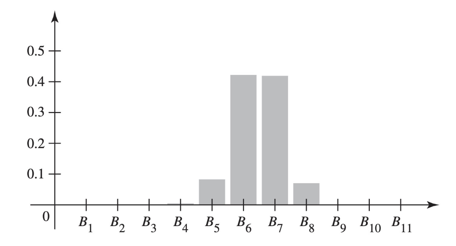
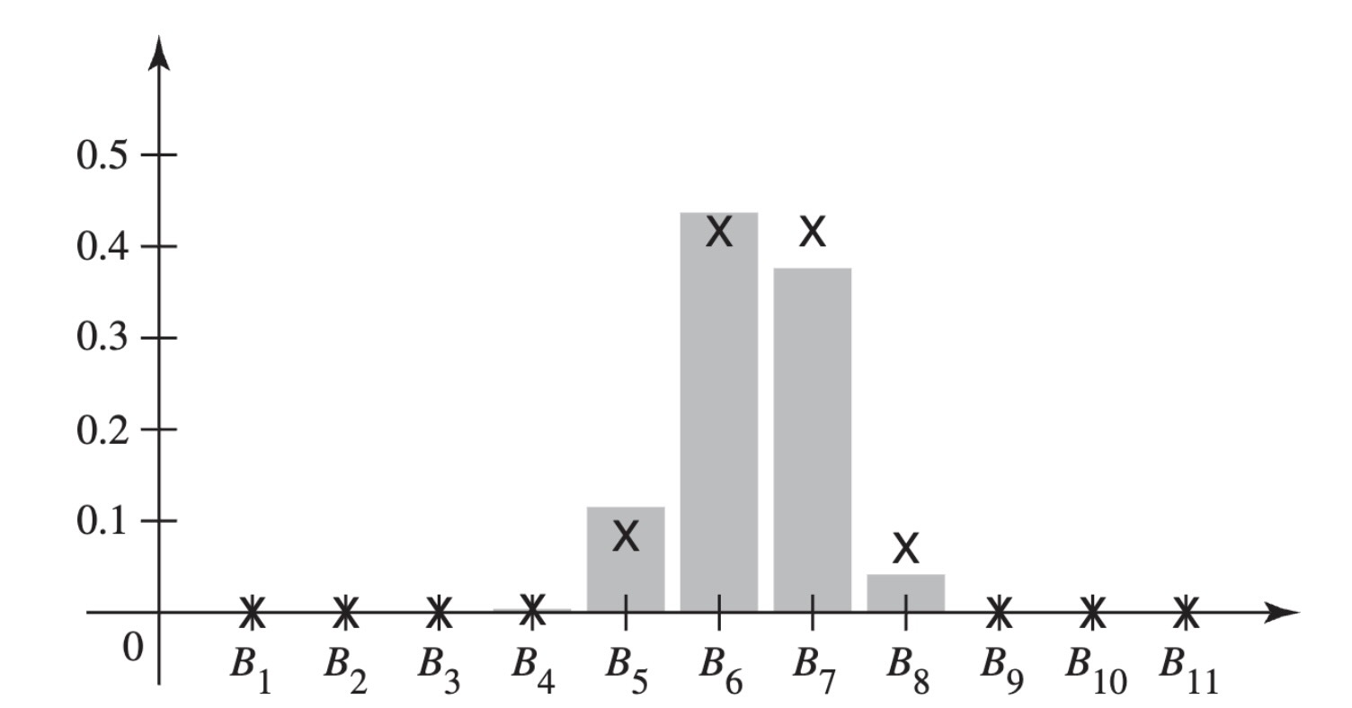
Figure 2.3: The posterior probabilities of partition elements after 40 patients in Example 2.30.

Figure 2.4: The posterior probabilities of partition elements after 40 patients in Example 2.31. The X characters mark the values of the posterior probabilities calculated in Example 2.30.

Example 2.31 (Example 2.3.8: The Effect of Prior Probabilities) Consider the same clinical trial as in Example 2.30. This time, suppose that a different researcher has a different prior opinion about the value of $p$, the probability of success. This researcher believes the following prior probabilities:

Event	$B_1$	$B_2$	$B_3$	$B_4$	$B_5$	$B_6$	$B_7$	$B_8$	$B_9$	$B_{10}$	$B_{11}$
$p$	0.0	0.1	0.2	0.3	0.4	0.5	0.6	0.7	0.8	0.9	1.0
Prior prob.	0.00	0.19	0.19	0.17	0.14	0.11	0.09	0.06	0.04	0.01	0.00

We can recalculate the posterior probabilities using Bayes’ theorem, and we get the values pictured in Figure 2.4. To aid comparison, the posterior probabilities from Example 2.30 are also plotted in Figure 2.4 using the symbol X. One can see how close the two sets of posterior probabilities are despite the large differences between the prior probabilities. If there had been fewer patients observed, there would have been larger differences between the two sets of posterior probabilites because the observed events would have provided less information. (See Exercise 2.53 in this section.)

2.3.5 Summary

Bayes’ theorem tells us how to compute the conditional probability of each event in a partition given an observed event $A$. A major use of partitions is to divide the sample space into small enough pieces so that a collection of events of interest become conditionally independent given each event in the partition.

2.3.6 Exercises

Exercise 2.42 (Exercise 2.3.1) Suppose that $k$ events $B_1, \ldots, B_k$ form a partition of the sample space $S$. For $i = 1, \ldots, k$, let $\Pr(B_i)$ denote the prior probability of $B_i$. Also, for each event $A$ such that $\Pr(A) > 0$, let $\Pr(B_i \mid A)$ denote the posterior probability of $B_i$ given that the event $A$ has occurred. Prove that if $\Pr(B_1 \mid A) < \Pr(B_1)$, then $\Pr(B_i \mid A) > \Pr(B_i)$ for at least one value of $i$ ($i = 2, \ldots, k$).

Exercise 2.43 (Exercise 2.3.2) Consider again the conditions of Example 2.27 in this section, in which an item was selected at random from a batch of manufactured items and was found to be defective. For which values of $i$ ($i = 1, 2, 3$) is the posterior probability that the item was produced by machine $M_i$ larger than the prior probability that the item was produced by machine $M_i$?

Exercise 2.44 (Exercise 2.3.3) Suppose that in Example 2.27 in this section, the item selected at random from the entire lot is found to be nondefective. Determine the posterior probability that it was produced by machine $M_2$.

Exercise 2.45 (Exercise 2.3.4) A new test has been devised for detecting a particular type of cancer. If the test is applied to a person who has this type of cancer, the probability that the person will have a positive reaction is 0.95 and the probability that the person will have a negative reaction is 0.05. If the test is applied to a person who does not have this type of cancer, the probability that the person will have a positive reaction is 0.05 and the probability that the person will have a negative reaction is 0.95. Suppose that in the general population, one person out of every 100,000 people has this type of cancer. If a person selected at random has a positive reaction to the test, what is the probability that he has this type of cancer?

Exercise 2.46 (Exercise 2.3.5) In a certain city, 30 percent of the people are Conservatives, 50 percent are Liberals, and 20 percent are Independents. Records show that in a particular election, 65 percent of the Conservatives voted, 82 percent of the Liberals voted, and 50 percent of the Independents voted. If a person in the city is selected at random and it is learned that she did not vote in the last election, what is the probability that she is a Liberal?

Exercise 2.47 (Exercise 2.3.6) Suppose that when a machine is adjusted properly, 50 percent of the items produced by it are of high quality and the other 50 percent are of medium quality. Suppose, however, that the machine is improperly adjusted during 10 percent of the time and that, under these conditions, 25 percent of the items produced by it are of high quality and 75 percent are of medium quality.

Suppose that five items produced by the machine at a certain time are selected at random and inspected. If four of these items are of high quality and one item is of medium quality, what is the probability that the machine was adjusted properly at that time?
Suppose that one additional item, which was produced by the machine at the same time as the other five items, is selected and found to be of medium quality. What is the new posterior probability that the machine was adjusted properly?

Exercise 2.48 (Exercise 2.3.7) Suppose that a box contains five coins and that for each coin there is a different probability that a head will be obtained when the coin is tossed. Let $p_i$ denote the probability of a head when the $i$th coin is tossed ($i = 1, \ldots, 5$), and suppose that $p_1 = 0$, $p_2 = 1/4$, $p_3 = 1/2$, $p_4 = 3/4$, and $p_5 = 1$.

Suppose that one coin is selected at random from the box and when it is tossed once, a head is obtained. What is the posterior probability that the $i$th coin was selected ($i = 1, \ldots, 5$)?
If the same coin were tossed again, what would be the probability of obtaining another head?
If a tail had been obtained on the first toss of the selected coin and the same coin were tossed again, what would be the probability of obtaining a head on the second toss?

Exercise 2.49 (Exercise 2.3.8) Consider again the box containing the five different coins described in Exercise 2.48. Suppose that one coin is selected at random from the box and is tossed repeatedly until a head is obtained. a. If the first head is obtained on the fourth toss, what is the posterior probability that the $i$th coin was selected ($i = 1, \ldots, 5$)? b. If we continue to toss the same coin until another head is obtained, what is the probability that exactly three additional tosses will be required?

Exercise 2.50 (Exercise 2.3.9) Consider again the conditions of Exercise 2.14 in Section 2.1. Suppose that several parts will be observed and that the different parts are conditionally independent given each of the three states of repair of the machine. If seven parts are observed and exactly one is defective, compute the posterior probabilities of the three states of repair.

Exercise 2.51 (Exercise 2.3.10) Consider again the conditions of Example 2.28, in which the phenotype of an individual was observed and found to be the dominant trait. For which values of $i$ ($i = 1, \ldots, 6$) is the posterior probability that the parents have the genotypes of event $B_i$ smaller than the prior probability that the parents have the genotyes of event $B_i$?

Exercise 2.52 (Exercise 2.3.11) Suppose that in Example 2.28 the observed individual has the recessive trait. Determine the posterior probability that the parents have the genotypes of event $B_4$.

Exercise 2.53 (Exercise 2.3.12) In the clinical trial in Examples 2.30 and 2.31, suppose that we have only observed the first five patients and three of the five had been successes. Use the two different sets of prior probabilities from Examples 2.30 and 2.31 to calculate two sets of posterior probabilities. Are these two sets of posterior probabilities as close to each other as were the two in Examples 2.30 and 2.31? Why or why not?

Exercise 2.54 (Exercise 2.3.13) Suppose that a box contains one fair coin and one coin with a head on each side. Suppose that a coin is drawn at random from this box and that we begin to flip the coin. In Equation 2.13 and Equation 2.14, we computed the conditional probability that the coin was fair given that the first two flips both produce heads.

Suppose that the coin is flipped a third time and another head is obtained. Compute the probability that the coin is fair given that all three flips produced heads.
Suppose that the coin is flipped a fourth time and the result is tails. Compute the posterior probability that the coin is fair.

Exercise 2.55 (Exercise 2.3.14) Consider again the conditions of Exercise 2.40 in Section 2.2. Assume that $\Pr(B) = 0.4$. Let $A$ be the event that exactly 8 out of 11 programs compiled. Compute the conditional probability of $B$ given $A$.

Exercise 2.56 (Exercise 2.3.15) Use the prior probabilities in Example 2.31 for the events $B_1, \ldots, B_{11}$. Let $E_1$ be the event that the first patient is a success. Compute the probability of $E_1$ and explain why it is so much less than the value computed in Example 2.30.

Exercise 2.57 (Exercise 2.3.16) Consider a machine that produces items in sequence. Under normal operating conditions, the items are independent with probability 0.01 of being defective. However, it is possible for the machine to develop a “memory” in the following sense: After each defective item, and independent of anything that happened earlier, the probability that the next item is defective is $2/5$. After each nondefective item, and independent of anything that happened earlier, the probability that the next item is defective is $1/165$.

Assume that the machine is either operating normally for the whole time we observe or has a memory for the whole time that we observe. Let $B$ be the event that the machine is operating normally, and assume that $\Pr(B) = 2/3$. Let $D_i$ be the event that the $i$th item inspected is defective. Assume that $D_1$ is independent of $B$.

Prove that $\Pr(D_i) = 0.01$ for all $i$. Hint: Use induction.
Assume that we observe the first six items and the event that occurs is $E = D_1^c \cap D_2^c \cap D_3 \cap D_4 \cap D_5^c \cap D_6^c$. That is, the third and fourth items are defective, but the other four are not. Compute $\Pr(B \mid D)$.

2.4 The Gambler’s Ruin Problem

Consider two gamblers with finite resources who repeatedly play the same game against each other. Using the tools of conditional probability, we can calculate the probability that each of the gamblers will eventually lose all of his money to the opponent.

2.4.1 Statement of the Problem

Suppose that two gamblers $A$ and $B$ are playing a game against each other. Let $p$ be a given number ($0 < p < 1$), and suppose that on each play of the game, the probability that gambler $A$ will win one dollar from gambler $B$ is $p$ and the probability that gambler $B$ will win one dollar from gambler $A$ is $1 − p$. Suppose also that the initial fortune of gambler $A$ is $i$ dollars and the initial fortune of gambler $B$ is $k − i$ dollars, where $i$ and $k − i$ are given positive integers. Thus, the total fortune of the two gamblers is $k$ dollars. Finally, suppose that the gamblers play the game repeatedly and independently until the fortune of one of them has been reduced to 0 dollars. Another way to think about this problem is that $B$ is a casino and $A$ is a gambler who is determined to quit as soon he wins $k − i$ dollars from the casino or when he goes broke, whichever comes first.

We shall now consider this game from the point of view of gambler $A$. His initial fortune is $i$ dollars and on each play of the game his fortune will either increase by one dollar with a probability of $p$ or decrease by one dollar with a probability of $1 − p$. If $p > 1/2$, the game is favorable to him; if $p < 1/2$, the game is unfavorable to him; and if $p = 1/2$, the game is equally favorable to both gamblers. The game ends either when the fortune of gambler $A$ reaches $k$ dollars, in which case gambler $B$ will have no money left, or when the fortune of gambler $A$ reaches 0 dollars. The problem is to determine the probability that the fortune of gambler $A$ will reach $k$ dollars before it reaches 0 dollars. Because one of the gamblers will have no money left at the end of the game, this problem is called the Gambler’s Ruin problem.

2.4.2 Solution of the Problem

We shall continue to assume that the total fortune of the gamblers $A$ and $B$ is $k$ dollars, and we shall let $a_i$ denote the probability that the fortune of gambler $A$ will reach $k$ dollars before it reaches 0 dollars, given that his initial fortune is $i$ dollars. We assume that the game is the same each time it is played and the plays are independent of each other. It follows that, after each play, the Gambler’s Ruin problem essentially starts over with the only change being that the initial fortunes of the two gamblers have changed. In particular, for each $j = 0, \ldots, k$, each time that we observe a sequence of plays that lead to gambler $A$’s fortune being $j$ dollars, the conditional probability, given such a sequence, that gambler $A$ wins is $a_j$. If gambler $A$’s fortune ever reaches 0, then gambler $A$ is ruined, hence $a_0 = 0$. Similarly, if his fortune ever reaches $k$, then gambler $A$ has won, hence $a_k = 1$. We shall now determine the value of $a_i$ for $i = 1, \ldots, k-1$.

Let $A_1$ denote the event that gambler $A$ wins one dollar on the first play of the game, let $B_1$ denote the event that gambler $A$ loses one dollar on the first play of the game, and let $W$ denote the event that the fortune of gambler $A$ ultimately reaches $k$ dollars before it reaches 0 dollars. Then

\[ \begin{align*} \Pr(W) &= \Pr(A_1)\Pr(W \mid A_1) + \Pr(B_1)\Pr(W \mid B_1) \\ &= p \Pr(W \mid A_1) + (1-p)\Pr(W \mid B_1). \end{align*} \tag{2.18}\]

Since the initial fortune of gambler $A$ is $i$ dollars ($i = 1, \ldots, k-1$), then $\Pr(W) = a_i$. Furthermore, if gambler $A$ wins one dollar on the first play of the game, then his fortune becomes $i + 1$ dollars and the conditional probability $\Pr(W \mid A_1)$ that his fortune will ultimately reach $k$ dollars is therefore $a_{i+1}$. If $A$ loses one dollar on the first play of the game, then his fortune becomes $i − 1$ dollars and the conditional probability $\Pr(W \mid B_1)$ that his fortune will ultimately reach $k$ dollars is therefore $a_{i−1}. Hence, by Equation 2.18,

\[ a_i = pa_{i+1} + (1-p)a_{i-1}. \tag{2.19}\]

We shall let $i = 1, \ldots, k-1$ in Equation 2.19. Then, since $a_0 = 0$ and $a_k = 1$, we obtain the following $k − 1$ equations:

\[ \begin{align*} a_1 &= pa_2, \\ a_2 &= pa_3 + (1-p)a_1, \\ a_3 &= pa_4 + (1-p)a_2, \\ &\vdots \\ a_{k-2} &= pa_{k-1} + (1-p)a_{k-3}, \\ a_{k-1} &= p + (1-p)a_{k-2}. \end{align*} \tag{2.20}\]

If the value of $a_i$ on the left side of the $i$th equation is rewritten in the form $p a_i + (1 − p)a_i$ and some elementary algebra is performed, then these $k − 1$ equations can be rewritten as follows:

\[ \begin{align*} a_2 - a_1 &= \frac{1-p}{p}a_1, \\ a_3 - a_2 &= \frac{1-p}{p}(a_2 - a_1) = \left(\frac{1-p}{p}\right)^2a_1, \\ a_4 - a_3 &= \frac{1-p}{p}(a_3 - a_2) = \left(frac{1-p}{p}\right)^3a_1, \\ &\vdots \\ a_{k-1} - a_{k-2} &= \frac{1-p}{p}(a_{k-2} - a_{k-3}) = \left(\frac{1-p}{p}\right)^{k-2}a_1, \\ 1 - a_{k-1} &= \frac{1-p}{p}(a_{k-1} - a_{k-2}) = \left(\frac{1-p}{p}\right)^{k-1}a_1. \end{align*} \tag{2.21}\]

By equating the sum of the left sides of these $k − 1$ equations with the sum of the right sides, we obtain the relation

\[ 1 - a_1 = a_1 \sum_{i=1}^{k-1} \left(\frac{1-p}{p}\right)^i \tag{2.22}\]

Solution for a Fair Game: Suppose first that $p = 1/2$. Then $(1 − p)/p = 1$, and it follows from Equation 2.22 that $1 − a_1 = (k − 1)a_1$, from which $a_1= 1/k$. In turn, it follows from the first equation in Equation 2.21 that $a_2 = 2/k$, it follows from the second equation in Equation 2.21 that $a_3 = 3/k$, and so on. In this way, we obtain the following complete solution when $p = 1/2$:

\[ a_i = \frac{i}{k} \; \text{ for }i = 1, \ldots, k-1. \tag{2.23}\]

Example 2.32 (Example 2.4.1: The Probability of Winning in a Fair Game) Suppose that $p = 1/2$, in which case the game is equally favorable to both gamblers; and suppose that the initial fortune of gambler $A$ is 98 dollars and the initial fortune of gambler $B$ is just two dollars. In this example, $i = 98$ and $k = 100$. Therefore, it follows from Equation 2.23 that there is a probability of 0.98 that gambler $A$ will win two dollars from gambler $B$ before gambler $B$ wins 98 dollars from gambler $A$.

Solution for an Unfair Game: Suppose now that $p \neq 1/2$. Then Equation 2.22 can be rewritten in the form

\[ 1 - a_1 = a_1 \frac{ \left(\frac{1-p}{p}\right)^k - \left(\frac{1-p}{p}\right) }{ \left(\frac{1-p}{p}\right) - 1 }. \tag{2.24}\]

Hence,

\[ a_1 = \frac{ \left(\frac{1-p}{p}\right) - 1 }{ \left(\frac{1-p}{p}\right)^k - 1 }. \tag{2.25}\]

Each of the other values of $a_i$ for $i = 2, \ldots, k-1$ can now be determined in turn from the equations in Equation 2.21. In this way, we obtain the following complete solution:

\[ a_i = \frac{ \left(\frac{1-p}{p}\right)^i - 1 }{ \left(\frac{1-p}{p}\right)^k - 1 } \; \text{ for }i = 1, \ldots, k-1. \tag{2.26}\]

Example 2.33 (Example 2.4.2: The Probability of Winning in an Unfavorable Game) Suppose that $p = 0.4$, in which case the probability that gambler $A$ will win one dollar on any given play is smaller than the probability that he will lose one dollar. Suppose also that the initial fortune of gambler $A$ is 99 dollars and the initial fortune of gambler $B$ is just one dollar. We shall determine the probability that gambler $A$ will win one dollar from gambler $B$ before gambler $B$ wins 99 dollars from gambler $A$.

In this example, the required probability $a_i$ is given by Equation 2.26, in which $(1-p)/p = 3/2$, $i = 99$, and $k = 100$. Therefore,

\[ a_i = \frac{ \left(\frac{3}{2}\right)^{99} - 1 }{ \left(\frac{3}{2}\right)^{100} - 1 } \approx \frac{1}{3/2} = \frac{2}{3}. \]

Hence, although the probability that gambler $A$ will win one dollar on any given play is only 0.4, the probability that he will win one dollar before he loses 99 dollars is approximately $2/3$.

2.4.3 Summary

We considered a gambler and an opponent who each start with finite amounts of money. The two then play a sequence of games against each other until one of them runs out of money. We were able to calculate the probability that each of them would be the first to run out as a function of the probability of winning the game and of how much money each has at the start.

2.4.4 Exercises

Exercise 2.58 (Exercise 2.4.1) Consider the unfavorable game in Example 2.33. This time, suppose that the initial fortune of gambler $A$ is $i$ dollars with $i \leq 98$. Suppose that the initial fortune of gambler $B$ is $100 − i$ dollars. Show that the probability is greater than $1/2$ that gambler $A$ loses $i$ dollars before winning $100 − i$ dollars.

Exercise 2.59 (Exercise 2.4.2) Consider the following three different possible conditions in the gambler’s ruin problem:

The initial fortune of gambler $A$ is two dollars, and the initial fortune of gambler $B$ is one dollar.
The initial fortune of gambler $A$ is 20 dollars, and the initial fortune of gambler $B$ is 10 dollars.
The initial fortune of gambler $A$ is 200 dollars, and the initial fortune of gambler $B$ is 100 dollars.

Suppose that $p = 1/2$. For which of these three conditions is there the greatest probability that gambler $A$ will win the initial fortune of gambler $B$ before he loses his own initial fortune?

Exercise 2.60 (Exercise 2.4.3) Consider again the three different conditions (a), (b), and (c) given in Exercise 2.59, but suppose now that $p < 1/2$. For which of these three conditions is there the greatest probability that gambler $A$ will win the initial fortune of gambler $B$ before he loses his own initial fortune?

Exercise 2.61 (Exercise 2.4.4) Consider again the three different conditions (a), (b), and (c) given in Exercise 2.59, but suppose now that $p > 1/2$. For which of these three conditions is there the greatest probability that gambler $A$ will win the initial fortune of gambler $B$ before he loses his own initial fortune?

Exercise 2.62 (Exercise 2.4.5) Suppose that on each play of a certain game, a person is equally likely to win one dollar or lose one dollar. Suppose also that the person’s goal is to win two dollars by playing this game. How large an initial fortune must the person have in order for the probability to be at least 0.99 that she will achieve her goal before she loses her initial fortune?

Exercise 2.63 (Exercie 2.4.6) Suppose that on each play of a certain game, a person will either win one dollar with probability $2/3$ or lose one dollar with probability $1/3$. Suppose also that the person’s goal is to win two dollars by playing this game. How large an initial fortune must the person have in order for the probability to be at least 0.99 that he will achieve his goal before he loses his initial fortune?

Exercise 2.64 (Exercise 2.4.7) Suppose that on each play of a certain game, a person will either win one dollar with probability $1/3$ or lose one dollar with probability $2/3$. Suppose also that the person’s goal is to win two dollars by playing this game. Show that no matter how large the person’s initial fortune might be, the probability that she will achieve her goal before she loses her initial fortune is less than $1/4$.

Exercise 2.65 (Exercise 2.4.8) Suppose that the probability of a head on any toss of a certain coin is $p$ ($0 < p < 1$), and suppose that the coin is tossed repeatedly. Let $X_n$ denote the total number of heads that have been obtained on the first $n$ tosses, and let $Y_n = n − X_n$ denote the total number of tails on the first $n$ tosses. Suppose that the tosses are stopped as soon as a number $n$ is reached such that either $X_n = Y_n + 3$ or $Y_n = X_n + 3$. Determine the probability that $X_n = Y_n + 3$ when the tosses are stopped.

Exercise 2.66 (Exercise 2.4.9) Suppose that a certain box $A$ contains five balls and another box $B$ contains 10 balls. One of these two boxes is selected at random, and one ball from the selected box is transferred to the other box. If this process of selecting a box at random and transferring one ball from that box to the other box is repeated indefinitely, what is the probability that box $A$ will become empty before box $B$ becomes empty?

2.5 Supplementary Exercises

Exercise 2.67 (Exercise 2.5.1) Suppose that $A$, $B$, and $D$ are any three events such that $\Pr(A \mid D) \geq \Pr(B \mid D)$ and $\Pr(A \mid D^c) \geq \Pr(B \mid D^c)$. Prove that $\Pr(A) \geq \Pr(B)$.

Exercise 2.68 (Exercise 2.5.2) Suppose that a fair coin is tossed repeatedly and independently until both a head and a tail have appeared at least once.

Describe the sample space of this experiment.
What is the probability that exactly three tosses will be required?

Exercise 2.69 (Exercise 2.5.3) Suppose that $A$ and $B$ are events such that $\Pr(A) = 1/3$, $\Pr(B) = 1/5$, and $\Pr(A \mid B) + \Pr(B \mid A) = 2/3$. Evaluate $\Pr(A^c \cup B^c)$.

Exercise 2.70 (Exercise 2.5.4) Suppose that $A$ and $B$ are independent events such that $\Pr(A) = 1/3$ and $\Pr(B) > 0$. What is the value of $\Pr(A \cup B^c \mid B)$?

Exercise 2.71 (Exercise 2.5.5) Suppose that in 10 rolls of a balanced die, the number 6 appeared exactly three times. What is the probability that the first three rolls each yielded the number 6?

Exercise 2.72 (Exercise 2.5.6) Suppose that $A$, $B$, and $D$ are events such that $A$ and $B$ are independent, $\Pr(A \cap B \cap D) = 0.04$, $\Pr(D \mid A \cap B) = 0.25$, and $\Pr(B) = 4 \Pr(A)$. Evaluate $\Pr(A \cup B)$.

Exercise 2.73 (Exercise 2.5.7) Suppose that the events $A$, $B$, and $C$ are mutually independent. Under what conditions are $A^c$, $B^c$, and $C^c$ mutually independent?

Exercise 2.74 (Exercise 2.5.8) Suppose that the events $A$ and $B$ are disjoint and that each has positive probability. Are $A$ and $B$ independent?

Exercise 2.75 (Exercise 2.5.9) Suppose that $A$, $B$, and $C$ are three events such that $A$ and $B$ are disjoint, $A$ and $C$ are independent, and $B$ and $C$ are independent. Suppose also that $4\Pr(A) = 2\Pr(B) = \Pr(C) > 0$ and $\Pr(A \cup B \cup C) = 5\Pr(A)$. Determine the value of $\Pr(A)$.

Exercise 2.76 (Exercise 2.5.10) Suppose that each of two dice is loaded so that when either die is rolled, the probability that the number $k$ will appear is 0.1 for $k = 1$, $2$, $5$, or $6$ and is 0.3 for $k = 3$ or $4$. If the two loaded dice are rolled independently, what is the probability that the sum of the two numbers that appear will be 7?

Exercise 2.77 (Exercise 2.5.11) Suppose that there is a probability of $1/50$ that you will win a certain game. If you play the game 50 times, independently, what is the probability that you will win at least once?

Exercise 2.78 (Exercise 2.5.12) Suppose that a balanced die is rolled three times, and let $X_i$ denote the number that appears on the ith roll ($i = 1, 2, 3$). Evaluate $\Pr(X_1 > X_2 > X_3)$.

Exercise 2.79 (Exercise 2.5.13) Three students $A$, $B$, and $C$ are enrolled in the same class. Suppose that $A$ attends class 30 percent of the time, $B$ attends class 50 percent of the time, and $C$ attends class 80 percent of the time. If these students attend class independently of each other, what is (a) the probability that at least one of them will be in class on a particular day and (b) the probability that exactly one of them will be in class on a particular day?

Exercise 2.80 (Exercise 2.5.14) Consider the World Series of baseball, as described in Exercise 2.33 of Section 2.2. If there is probability $p$ that team $A$ will win any particular game, what is the probability that it will be necessary to play seven games in order to determine the winner of the Series?

Exercise 2.81 (Exercise 2.5.15) Suppose that three red balls and three white balls are thrown at random into three boxes and and that all throws are independent. What is the probability that each box contains one red ball and one white ball?

Exercise 2.82 (Exercise 2.5.16) If five balls are thrown at random into $n$ boxes, and all throws are independent, what is the probability that no box contains more than two balls?

Exercise 2.83 (Exercise 2.5.17) Bus tickets in a certain city contain four numbers, $U$, $V$, $W$, and $X$. Each of these numbers is equally likely to be any of the 10 digits $0, 1, \ldots, 9$, and the four numbers are chosen independently. A bus rider is said to be lucky if $U + V = W + X$. What proportion of the riders are lucky?

Exercise 2.84 (Exercise 2.5.18) A certain group has eight members. In January, three members are selected at random to serve on a committee. In February, four members are selected at random and independently of the first selection to serve on another committee. In March, five members are selected at random and independently of the previous two selections to serve on a third committee. Determine the probability that each of the eight members serves on at least one of the three committees.

Exercise 2.85 (Exercise 2.5.19) For the conditions of Exercise 2.84, determine the probability that two particular members $A$ and $B$ will serve together on at least one of the three committees.

Exercise 2.86 (Exercise 2.5.20) Suppose that two players $A$ and $B$ take turns rolling a pair of balanced dice and that the winner is the first player who obtains the sum of 7 on a given roll of the two dice. If $A$ rolls first, what is the probability that $B$ will win?

Exercise 2.87 (Exercise 2.5.21) Three players $A$, $B$, and $C$ take turns tossing a fair coin. Suppose that $A$ tosses the coin first, $B$ tosses second, and $C$ tosses third; and suppose that this cycle is repeated indefinitely until someone wins by being the first player to obtain a head. Determine the probability that each of three players will win.

Exercise 2.88 (Exercise 2.5.22) Suppose that a balanced die is rolled repeatedly until the same number appears on two successive rolls, and let $X$ denote the number of rolls that are required. Determine the value of $\Pr(X = x)$, for $x = 2, 3, \ldots$.

Exercise 2.89 (Exercise 2.5.23) Suppose that 80 percent of all statisticians are shy, whereas only 15 percent of all economists are shy. Suppose also that 90 percent of the people at a large gathering are economists and the other 10 percent are statisticians. If you meet a shy person at random at the gathering, what is the probability that the person is a statistician?

Exercise 2.90 (Exercise 2.5.24) Dreamboat cars are produced at three different factories $A$, $B$, and $C$. Factory $A$ produces 20 percent of the total output of Dreamboats, $B$ produces 50 percent, and $C$ produces 30 percent. However, 5 percent of the cars produced at $A$ are lemons, 2 percent of those produced at $B$ are lemons, and 10 percent of those produced at $C$ are lemons. If you buy a Dreamboat and it turns out to be a lemon, what is the probability that it was produced at factory $A$?

Exercise 2.91 (Exercise 2.5.25) Suppose that 30 percent of the bottles produced in a certain plant are defective. If a bottle is defective, the probability is 0.9 that an inspector will notice it and remove it from the filling line. If a bottle is not defective, the probability is 0.2 that the inspector will think that it is defective and remove it from the filling line.

If a bottle is removed from the filling line, what is the probability that it is defective?
If a customer buys a bottle that has not been removed from the filling line, what is the probability that it is defective?

Exercise 2.92 (Exercise 2.5.26) Suppose that a fair coin is tossed until a head is obtained and that this entire experiment is then performed independently a second time. What is the probability that the second experiment requires more tosses than the first experiment?

Exercise 2.93 (Exercise 2.5.27) Suppose that a family has exactly $n$ children ($n \geq 2$). Assume that the probability that any child will be a girl is $1/2$ and that all births are independent. Given that the family has at least one girl, determine the probability that the family has at least one boy.

Exercise 2.94 (Exercise 2.5.28) Suppose that a fair coin is tossed independently $n$ times. Determine the probability of obtaining exactly $n - 1$ heads, given (a) that at least $n − 2$ heads are obtained and (b) that heads are obtained on the first $n − 2$ tosses.

Exercise 2.95 (Exercise 2.5.29) Suppose that 13 cards are selected at random from a regular deck of 52 playing cards.

If it is known that at least one ace has been selected, what is the probability that at least two aces have been selected?
If it is known that the ace of hearts has been selected, what is the probability that at least two aces have been selected?

Exercise 2.96 (Exercise 2.5.30) Suppose that $n$ letters are placed at random in $n$ envelopes, as in the matching problem of Section 1.10, and let $q_n$ denote the probability that no letter is placed in the correct envelope. Show that the probability that exactly one letter is placed in the correct envelope is $q_{n−1}$.

Exercise 2.97 (Exercise 2.5.31) Consider again the conditions of Exercise 2.96. Show that the probability that exactly two letters are placed in the correct envelopes is $(1/2)q_{n−2}$.

Exercise 2.98 (Exercise 2.5.32) Consider again the conditions of Exercise 2.24 of Section 2.2. If exactly one of the two students $A$ and $B$ is in class on a given day, what is the probability that it is $A$?

Exercise 2.99 (Exercise 2.5.33) Consider again the conditions of Exercise 1.83 of Section 1.10. If a family selected at random from the city subscribes to exactly one of the three newspapers $A$, $B$, and $C$, what is the probability that it is $A$?

Exercise 2.100 (Exercise 2.5.34) Three prisoners $A$, $B$, and $C$ on death row know that exactly two of them are going to be executed, but they do not know which two. Prisoner $A$ knows that the jailer will not tell him whether or not he is going to be executed. He therefore asks the jailer to tell him the name of one prisoner other than $A$ himself who will be executed. The jailer responds that $B$ will be executed. Upon receiving this response, Prisoner $A$ reasons as follows: Before he spoke to the jailer, the probability was $2/3$ that he would be one of the two prisoners executed. After speaking to the jailer, he knows that either he or prisoner $C$ will be the other one to be executed. Hence, the probability that he will be executed is now only $1/2$. Thus, merely by asking the jailer his question, the prisoner reduced the probability that he would be executed from $2/3$ to $1/2$, because he could go through exactly this same reasoning regardless of which answer the jailer gave. Discuss what is wrong with prisoner $A$’s reasoning.

Exercise 2.101 (Exercise 2.5.35) Suppose that each of two gamblers $A$ and $B$ has an initial fortune of 50 dollars, and that there is probability $p$ that gambler $A$ will win on any single play of a game against gambler $B$. Also, suppose either that one gambler can win one dollar from the other on each play of the game or that they can double the stakes and one can win two dollars from the other on each play of the game. Under which of these two conditions does $A$ have the greater probability of winning the initial fortune of $B$ before losing her own for each of the following conditions: (a) $p < 1/2$; (b) $p > 1/2$; (c) $p = 1/2$?

Exercise 2.102 (Exercise 2.5.36) A sequence of $n$ job candidates is prepared to interview for a job. We would like to hire the best candidate, but we have no information to distinguish the candidates before we interview them. We assume that the best candidate is equally likely to be each of the $n$ candidates in the sequence before the interviews start. After the interviews start, we are able to rank those candidates we have seen, but we have no information about where the remaining candidates rank relative to those we have seen. After each interview, it is required that either we hire the current candidate immediately and stop the interviews, or we must let the current candidate go and we never can call them back. We choose to interview as follows: We select a number $0 \leq r < n$ and we interview the first $r$ candidates without any intention of hiring them. Starting with the next candidate $r + 1$, we continue interviewing until the current candidate is the best we have seen so far. We then stop and hire the current candidate. If none of the candidates from $r + 1$ to $n$ is the best, we just hire candidate $n$. We would like to compute the probability that we hire the best candidate and we would like to choose $r$ to make this probability as large as possible. Let $A$ be the event that we hire the best candidate, and let $B_i$ be the event that the best candidate is in position $i$ in the sequence of interviews.

Let $i > r$. Find the probability that the candidate who is relatively the best among the first $i$ interviewed appears in the first $r$ interviews.
Prove that $\Pr(A \mid B_i) = 0$ for $i \leq r$ and $\Pr(A \mid B_i) = r/(i − 1)$ for $i > r$.
For fixed $r$, let $p_r$ be the probability of $A$ using that value of $r$. Prove that $p_r = (r/n)\sum_{i=r+1}^{n}(i-1)^{-1}$.
Let $q_r = p_r − p_{r−1}$ for $r = 1, \ldots, n - 1$, and prove that $q_r$ is a strictly decreasing function of $r$.
Show that a value of $r$ that maximizes $p_r$ is the last $r$ such that $q_r > 0$. (Hint: Write $p_r = p_0 + q_1 + \cdots + q_r$ for $r > 0$.)
For $n = 10$, find the value of $r$ that maximizes $p_r$, and find the corresponding $p_r$ value.

	\((AA, AA)\)	\((AA, Aa)\)	\((AA,aa)\)	\((Aa, Aa)\)	\((Aa, aa)\)	\((aa, aa)\)
Name of event	\(B_1\)	\(B_2\)	\(B_3\)	\(B_4\)	\(B_5\)	\(B_6\)
probability of \(B_i\)	\(1/16\)	\(1/4\)	\(1/8\)	\(1/4\)	\(1/4\)	\(1/16\)
\(\Pr(E \mid B_i)\)	1	1	1	\(3/4\)	\(1/2\)	0