Workshop Week 6: Midterm Coding Preview

DSAN 5650: Causal Inference for Computational Social Science
Summer 2026, Georgetown University

Class Sessions

Author

Affiliation

Jeff Jacobs

jj1088@georgetown.edu

Published

Friday, June 26, 2026

DSAN 5650 Week 6 Coding Workshop: Selective Transmission of Historical Documents

Loading and Exploring the Data

This question is going to feel a bit “in the weeds” at first – because it is – but points to the importance of the library of missing datasets which lurks behind any actually-existing dataset you may find! It also relates to Berkson’s Paradox, which will be the subject of Part 2 below.

Code

import pandas as pd
import numpy as np
import matplotlib.pyplot as plt
import seaborn as sns

import pymc as pm

Code

pub_url = "https://raw.githubusercontent.com/jpowerj/dsan-content/refs/heads/main/2025-sum-dsan5650/cahiers_official.csv"
pub_df = pd.read_csv(pub_url)
pub_df.head()

	village_name	published	huguenot
0	ARRAS (ARTOIS)	True	False
1	AURAY, REUNI A VANNES (SEN)	True	False
2	AUTUN	True	True
3	BOULAY, REUNI A SARREGUEMINES	True	True
4	CALAIS	True	False

As the following cell shows, there were 32 villages whose cahiers were deemed “exemplary” of the grievances of France as a whole:

Code

len(pub_df)

And, as the following cell makes clear, over 40% of these “exemplary” cahiers contained grievances about the treatment of French Protestants (Huguenots):

Code

pub_df['huguenot'].value_counts(normalize=True)

huguenot
False    0.59375
True     0.40625
Name: proportion, dtype: float64

[Question 1.1] Modeling the Published Documents

In the following code cell, use PyMC to create a generative model of the published cahiers as follows:

First, the model should include a variable p_hug, representing the overall probability that a given cahier contains a grievance related to treatment of Huguenots
Then, the model should include a village-specific variable huguenot, a binary variable which has the value 1 for villages whose cahier contains a grievance related to treatment of Huguenots, and 0 for villages whose cahier does not contain such a grievance.

p_hug and huguenot should be linked such that the probability of huguenot taking the value 1 is exactly p_hug – the included line of code at the end of the cell prints the model as a PGM, where there should be an arrow from the p_hug node to the huguenot node!

Code

village_idx, village_name = pub_df['village_name'].factorize()
print(village_idx)
print(village_name)

[ 0  1  2  3  4  5  6  7  8  9 10 11 12 13 14 15 16 17 18 19 20 21 22 23
 24 25 26 27 28 29 30 31]
Index(['ARRAS (ARTOIS)', 'AURAY, REUNI A VANNES (SEN)', 'AUTUN',
       'BOULAY, REUNI A SARREGUEMINES', 'CALAIS', 'CARCASSONNE',
       'CARIGNAN, REUNI A SEDAN', 'CHATEAU-SALINS, REUNI A SARREGUEMINES',
       'COMMINGES', 'COUTANCES, BAILLIAGE PRINCIPALE',
       'DIGNE, REUNI A FORCALQUIER', 'DOLE', 'DRAGUIGNAN, CENTRE DE REUNION',
       'FORCALQUIER, CENTRE DE REUNION', 'LAMARCHE, REUNI A BAR-LE-DUC',
       'LIMOGES', 'LONGWY, REUNI A METZ (BAILL)', 'LUNEVILLE, REUNI A NANCY',
       'MELUN', 'MONTREUIL-SUR-MER', 'NANCY, CENTRE DE REUNION', 'PAMIERS',
       'PARIS (HORS-LES-MURS)', 'REIMS', 'SARRELOUIS, REUNI A METZ (BAILL)',
       'SAUMUR', 'SENLIS', 'SENS', 'THIAUCOURT, REUNI A BAR-LE-DUC',
       'TOULON, CENTRE DE REUNION', 'VERDUN, CENTRE DE REUNION',
       'VILLEFRANCHE (BEAUJOLAIS)'],
      dtype='str')

Code

# @title Q1.1-response
pub_coords = {
  'village': village_name
}
with pm.Model(coords=pub_coords) as pub_model:
  # Your code here: model the two random variables p_hug and huguenot as
  # described above
  huguenot_obs = pm.Data('huguenot_obs', pub_df['huguenot'], dims='village')
  p_hug = pm.Uniform('p_hug', lower=0, upper=1)
  huguenot = pm.Bernoulli('huguenot', p=p_hug, observed=huguenot_obs, dims='village')
  # p_hug = 

if pub_model is not None:
  display(pm.model_to_graphviz(pub_model))

[Question 1.2] Sampling from the Prior Distribution

Now, in the following code cell, sample from the prior predictive distribution using PyMC’s sample_prior_predictive() function, storing the result in a variable named pub_prior_idata. Once this variable is created correctly, the remaining provided code will construct a Pandas DataFrame and plot the distribution of p_hug:

Code

# @title Q1.2-response
# Your code here: create a variable pub_prior_idata containing the predictive prior
# distribution
pub_prior_idata = pm.sample(model=pub_model)

Initializing NUTS using jitter+adapt_diag...
Multiprocess sampling (4 chains in 4 jobs)
NUTS: [p_hug]

Sampling 4 chains for 1_000 tune and 1_000 draw iterations (4_000 + 4_000 draws total) took 1 seconds.

Code

pub_prior_idata

Code

# Convert to DataFrame
pub_prior_df = pub_prior_idata.posterior.ds.to_dataframe().reset_index().drop(columns="chain")
pub_prior_df

	draw	p_hug
0	0	0.318346
1	1	0.415620
2	2	0.415620
3	3	0.392720
4	4	0.437074
...	...	...
3995	995	0.242635
3996	996	0.333296
3997	997	0.448465
3998	998	0.461109
3999	999	0.313271

4000 rows × 2 columns

Code



# And plot
sns.kdeplot(
    x="p_hug", data=pub_prior_df, fill=True,
  #binwidth=0.05
);
plt.axvline(0.411)
plt.show()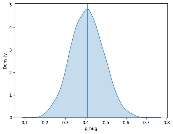

Code

import arviz as az

az.summary(pub_prior_idata)

	mean	sd	eti89_lb	eti89_ub	ess_bulk	ess_tail	r_hat	mcse_mean	mcse_sd
p_hug	0.408	0.081	0.28	0.54	1663	2150	1.00	0.002	0.0014

Inferring the Number of Cahiers Containing Huguenot Grievances

If the above code worked as intended, the following code cell should just take the pub_prior_idata variable you created and use it to infer the number of published cahiers (out of the 32 total that were chosen) containing Huguenot grievances (demonstrating how we can use your model to “jump” to a more coarse-grained level of “cahiers corpus” rather than just individual cahiers)

Code

# @title Q1.2-infer-num-cahiers
pub_prior_pred_df = pub_prior_idata.prior_predictive.to_dataframe().reset_index().drop(columns="chain")
sum_df = pub_prior_pred_df.groupby('draw')['huguenot'].sum().to_frame().reset_index()
sum_df.rename(columns={'huguenot': 'num_huguenot'}, inplace=True)
true_num_hug = len(pub_df[pub_df['huguenot']])

ax = pw.Brick(figsize=(4,2.5));
sns.histplot(
    x="num_huguenot", data=sum_df, ax=ax,
    discrete=True
);
ax.axvline(x=true_num_hug, ls='dashed', color='black', alpha=0.9);
ax.savefig()

[Question 1.3] Sampling from the Posterior Distribution

Now, let’s estimate the model parameters using the actual data! In the following code cell, use sample() (rather than sample_prior_predictive() to draw the actual Bayesian-optimized parameter values, storing the result in a variable named pub_post_idata.

If sampled correctly, the plot of the posterior distribution of p_hug generated by the included code should be centered around the true value of about 0.4.

Code

# @title Q1.3-response
# Your code here: use pm.sample() to estimate the *posterior* distribution from
# the data in pub_df

# Convert to DataFrame
pub_post_df = pub_post_idata.posterior.to_dataframe().reset_index()
pub_post_df = pub_post_df.groupby('draw')['p_hug'].mean().to_frame()
# And plot
ax = pw.Brick(figsize=(4, 2.5));
sns.kdeplot(
    x="p_hug", data=pub_post_df, ax=ax,
    fill=True
);
ax.axvline(x=pub_post_df['p_hug'].mean(), lw=1, ls='dashed', alpha=0.9);
ax.savefig()

[Question 1.4] Sampling from the Posterior Predictive Distribution

Now, drawing on the example code above which performed this coarse-graining on the prior predictive distribution (the code cell titled Q1.2-infer-num-cahiers), first use PyMC’s sample_posterior_predictive() function to sample the model’s posterior predictive distribution, then use it to generate a plot of the posterior predictive distribution of a variable you should name num_huguenot: the estimated number of cahiers mentioning Huguenot grievances given the learned parameters of your model.

Code

# @title Q1.4-response
with pub_model:
    pub_post_pred_idata = pm.sample_posterior_predictive(pub_post_idata, random_seed=5650)

Code

pub_post_pred_df = pub_post_pred_idata.posterior_predictive.to_dataframe().reset_index()
pub_post_pred_df = pub_post_pred_df[pub_post_pred_df['chain'] == 0].drop(columns="chain")
pub_post_pred_df

Code

post_sum_df = pub_post_pred_df.groupby('draw')['huguenot'].sum().to_frame().reset_index()
post_sum_df.rename(columns={'huguenot': 'num_huguenot'}, inplace=True)
post_sum_df

Code

true_num_hug = len(pub_df[pub_df['huguenot']])

ax = pw.Brick(figsize=(4,2.5));
sns.histplot(
    x="num_huguenot", data=post_sum_df, ax=ax,
    discrete=True
);
ax.axvline(x=true_num_hug, ls='dashed', color='black', alpha=0.9);
ax.savefig()

[Question 1.5] Accounting for Bias

However, this is where domain knowledge can come into play. To condense a long story into a nice neat narrative for this exam (since this is not a class about the French Revolution!), here are four quick stylized facts:

A popular interpretation of the French Revolution argues that it was a “bourgeois revolution”, meaning that it was in essence the seizure of power by budding capitalists away from the French monarchy.
For a bunch of reasons (like their connections with rich Germans who had adopted Protestantism centuries earlier), wealthy Huguenots were seen as possible “replacements” for the Catholic allies whom French Revolutionaries had alienated (e.g., by nationalizing all Church property and forcing Catholic priests to sign an oath of loyalty to the nation of France over Rome). However, many of them had fled in
In addition to the ~700,000 Huguenots, there was a mass influx of ~40,000 Protestants from the Netherlands, who were also among the wealthy elites of that country.
There was a guy named Jean-Paul Rabaut who you can think of as a “spokesman” for the Huguenot community of France during the crucial first 4 years of the French Revolution (until he was guillotined in 1793). Rabaut put Huguenot rights “on the agenda” as the president of the French National Assembly in 1790, and more generally could use his power to put Huguenot

These four facts put together hopefully help motivate the hypothesis that the French Revolutionaries – especially those involved in shaping the “public image” of the Revolution – had an interest in emphasizing the freedom that Protestants now had. Concretely, this led to the following law passed in December of 1790:

All persons born in a foreign country and descending in any degree of a French man or woman expatriated for religious reasons are declared French nationals (naturels français) and will benefit from rights attached to that quality if they come back to France, establish their domicile there and take the civic oath.

And so, the hypothesis just becomes that: the same collection of people who organized around Huguenot rights to push laws like this into being, also pushed to ensure that narratives of the French Revolution such as those embodied in document collections would emphasize the Huguenot struggle as much as possible.

Given all this, your job in this part is to model the possible bias in representation arising from this push: rather than modeling the distribution \(\Pr(\textsf{Huguenot})\) as independent of the distribution \(\Pr(\textsf{Published})\), you should now model an inflation factor representing how much the proportion of published cahiers mentioning Huguenots was inflated (or deflated!) relative to the total collection of cahiers.

In other words, your new model should have a variable named p_pub_nohug representing the probability of a cahier being published given that it does not contain a Huguenot-related grievance, and a variable named p_pub_hug representing the probability of a cahier that does contain a Huguenot-related grievance is published. (If it helps, think about the HW2C problem where you estimated disaster rates before and after a given change point – this problem should be a bit less complex than that, since you don’t need to estimate a changepoint in this case, just two separate \(\Pr(\textsf{Publish})\) distributions!)

Run the following code cell to load the data for all villages, then (a) use the prior-predictive distribution to generate plots of p_pub_nohug and p_pub_hug

Code

full_url = "https://raw.githubusercontent.com/jpowerj/dsan-content/refs/heads/main/2025-sum-dsan5650/cahiers_all.csv"
full_df = pd.read_csv(full_url)
full_df.head()

Code

len(full_df)

Code

hug_values = full_df['huguenot']
pub_values = full_df['published']
village_idx, village_names = full_df['village_name'].factorize()
coords = {'village': village_idx}
with pm.Model(coords=coords) as infl_model:
    # Your code here: model the probability of publication p_pub *with* and
    # *without* a Huguenot-related grievance, as described above!
    pass # Remove this pass statement once you've started coding your model!
if infl_model is not None:
    display(pm.model_to_graphviz(infl_model))

[Question 1.6] The Prior Predictive Distribution for `p_pub_nohug` and `p_pub_hug`

As in the published-only case from earlier, derive and plot the prior predictive distributions for these two parameters here. Name the derived prior data infl_prior_idata.

Code

# Your code here: store the prior data for the model as infl_prior_idata

# Convert to DataFrame
infl_prior_df = infl_prior_idata.prior.to_dataframe().reset_index().drop(columns='chain')
# Melt DataFrame to plot both p_pub_nohug and p_pub_hug within the same plot
infl_long_df = infl_prior_df[['draw','village','p_pub_nohug','p_pub_hug']].melt(id_vars=['draw','village'])
# And plot
ax = pw.Brick(figsize=(4, 2.5));
sns.kdeplot(
    x="value", hue="variable", data=infl_long_df, ax=ax,
    fill=True, bw_adjust=2,
);
ax.axvline(x=infl_prior_df['p_hug'].mean(), lw=1, ls='dashed', alpha=0.9);
ax.savefig()

[Question 1.7] The Posterior Distribution

You made it to the final step! Here, use PyMC’s sample() function to estimate the posterior distribution from the data in full_df loaded above, storing it in a variable named infl_post_idata:

Code

# @title Q1.7-response
# Your code here: estimate the *posterior* and store it in a variable named
# infl_post_idata

# Convert to DataFrame
infl_post_df = infl_post_idata.posterior.to_dataframe().reset_index()
# Extract only the first chain
infl_post_df = infl_post_df[infl_post_df['chain'] == 0]
# Melt as before
infl_post_long_df = infl_post_df[['draw','village','p_pub_nohug','p_pub_hug']].melt(id_vars=['draw','village'])
# And plot!
ax = pw.Brick(figsize=(4, 2.5));
sns.kdeplot(
    x="value", hue="variable", data=infl_post_long_df, ax=ax,
    fill=True, bw_adjust=2,
);
ax.savefig()

DSAN 5650 Week 6 Coding Workshop: Selective Transmission of Historical Documents

Loading and Exploring the Data

[Question 1.1] Modeling the Published Documents

[Question 1.2] Sampling from the Prior Distribution

Inferring the Number of Cahiers Containing Huguenot Grievances

[Question 1.3] Sampling from the Posterior Distribution

[Question 1.4] Sampling from the Posterior Predictive Distribution

[Question 1.5] Accounting for Bias

[Question 1.6] The Prior Predictive Distribution for p_pub_nohug and p_pub_hug

[Question 1.7] The Posterior Distribution

[Question 1.6] The Prior Predictive Distribution for `p_pub_nohug` and `p_pub_hug`