Workshop Week 5: PyMC’s idata (Inference Data) Structure

DSAN 5650: Causal Inference for Computational Social Science
Summer 2026, Georgetown University

Author

Affiliation

Jeff Jacobs

jj1088@georgetown.edu

DSAN 5650 Workshop 5: PyMC’s idata (Inference Data) Structure

1 “Customizable” Regression with PyMC

This is copied from Part 4 of Workshop 4, so that we can pick up where we left off last week, with our model of the impact of slave exports on present-day GDP, and the posterior distribution information stored as an idata object!

import pandas as pd
import numpy as np

import matplotlib.pyplot as plt
import seaborn as sns

import pymc as pm
import arviz as az
import xarray as xr
import preliz as pz

nunn_data_url = "https://github.com/jpowerj/dsan-content/raw/refs/heads/main/2026-sum-dsan5650/workshop01/slave_trade_QJE.dta"
country_df = pd.read_stata(nunn_data_url)
country_df.head()

	isocode	country	ln_maddison_pcgdp2000	ln_export_area	ln_export_pop	colony0	colony1	colony2	colony3	colony4	...	ln_avg_oil_pop	ln_avg_all_diamonds_pop	ln_pop_dens_1400	atlantic_distance_minimum	indian_distance_minimum	saharan_distance_minimum	red_sea_distance_minimum	ethnic_fractionalization	state_dev	land_area
0	AGO	Angola	6.670766	7.967494	14.399250	0.0	0.0	0.0	1.0	0.0	...	0.643126	-1.701396	-0.024917	5.668760	6.980571	4.925892	3.872354	0.7867	0.635	1.2500
1	BDI	Burundi	6.354370	1.140843	4.451658	0.0	0.0	0.0	0.0	1.0	...	-9.210340	-6.907755	3.036856	10.626214	2.570375	3.718742	2.215324	0.2951	0.995	0.0278
2	BEN	Benin	7.187657	8.304137	13.308970	0.0	0.0	1.0	0.0	0.0	...	-3.531555	-6.907755	1.214196	5.120652	9.233961	2.834785	3.901736	0.7872	0.695	0.1130
3	BFA	Burkina Faso	6.748760	6.413822	11.724286	0.0	0.0	1.0	0.0	0.0	...	-9.210340	-6.907755	0.908565	4.774938	9.299419	2.763519	4.239375	0.7377	0.338	0.2740
4	BWA	Botswana	8.377471	-2.302585	3.912023	0.0	1.0	0.0	0.0	0.0	...	-9.210340	2.186849	-2.075029	5.686335	5.764575	5.856533	4.299600	0.4102	0.893	0.6000

5 rows × 39 columns

1.1 Indexing in Pandas

By default, Pandas just assigns a numeric index which “labels” each row with coordinate values starting from 0 to (in this case) 51, so that the first country (Angola) has index 0, the second country (Burundi) has index 1, and so on:

country_df

	isocode	country	ln_maddison_pcgdp2000	ln_export_area	ln_export_pop	colony0	colony1	colony2	colony3	colony4	...	ln_avg_oil_pop	ln_avg_all_diamonds_pop	ln_pop_dens_1400	atlantic_distance_minimum	indian_distance_minimum	saharan_distance_minimum	red_sea_distance_minimum	ethnic_fractionalization	state_dev	land_area
0	AGO	Angola	6.670766	7.967494	14.399250	0.0	0.0	0.0	1.0	0.0	...	0.643126	-1.701396	-0.024917	5.668760	6.980571	4.925892	3.872354	0.7867	0.635	1.250000
1	BDI	Burundi	6.354370	1.140843	4.451658	0.0	0.0	0.0	0.0	1.0	...	-9.210340	-6.907755	3.036856	10.626214	2.570375	3.718742	2.215324	0.2951	0.995	0.027800
2	BEN	Benin	7.187657	8.304137	13.308970	0.0	0.0	1.0	0.0	0.0	...	-3.531555	-6.907755	1.214196	5.120652	9.233961	2.834785	3.901736	0.7872	0.695	0.113000
3	BFA	Burkina Faso	6.748760	6.413822	11.724286	0.0	0.0	1.0	0.0	0.0	...	-9.210340	-6.907755	0.908565	4.774938	9.299419	2.763519	4.239375	0.7377	0.338	0.274000
4	BWA	Botswana	8.377471	-2.302585	3.912023	0.0	1.0	0.0	0.0	0.0	...	-9.210340	2.186849	-2.075029	5.686335	5.764575	5.856533	4.299600	0.4102	0.893	0.600000
5	CAF	Central African Republic	6.472346	1.171314	8.052058	0.0	0.0	1.0	0.0	0.0	...	-9.210340	-1.849576	-0.473905	5.642056	8.772295	2.840084	2.293167	0.8295	0.144	0.623000
6	CIV	Ivory Coast	7.189922	5.096793	10.843699	0.0	0.0	1.0	0.0	0.0	...	-3.270892	-4.228216	0.472123	4.185696	9.457085	3.353074	4.793966	0.8204	0.082	0.322000
7	CMR	Cameroon	7.016610	4.944928	10.331063	0.0	0.0	1.0	0.0	0.0	...	-0.871162	-6.907755	1.020704	5.642056	8.772295	3.002548	3.051031	0.8635	0.316	0.475000
8	COG	Congo	7.702556	5.623267	12.391068	0.0	0.0	1.0	0.0	0.0	...	1.000878	-6.907755	-0.360961	5.527229	7.923528	3.697363	3.227007	0.8747	0.536	0.342000
9	COM	Comoros	6.364751	-2.302585	3.912023	0.0	0.0	1.0	0.0	0.0	...	-9.210340	-6.907755	-2.302585	10.130652	1.754229	4.845693	2.609506	0.0000	1.000	0.002170
10	CPV	Cape Verde Islands	7.482682	-2.302585	3.912023	0.0	0.0	0.0	1.0	0.0	...	-9.210340	-6.907755	-2.302585	3.646842	11.599784	3.481602	6.465437	0.4174	NaN	0.004030
11	DJI	Djibouti	7.005789	-1.661718	4.703024	0.0	0.0	1.0	0.0	0.0	...	-9.210340	-6.907755	-0.169874	14.407552	2.682206	2.350743	0.064390	0.7962	0.133	0.022000
12	DZA	Algeria	7.934514	3.257355	9.961392	0.0	0.0	1.0	0.0	0.0	...	0.913532	-6.907755	-0.404099	6.559232	14.912310	0.985090	3.654165	0.3394	0.990	2.380000
13	EGY	Egypt	7.979339	0.399917	5.477251	0.0	1.0	0.0	0.0	0.0	...	-0.361042	-6.907755	1.430923	16.392658	4.667312	0.430385	1.112658	0.1836	0.990	1.000000
14	ETH	Ethiopia	6.436151	7.078711	12.992780	1.0	0.0	0.0	0.0	0.0	...	-9.210340	-6.907755	0.355667	12.588990	2.705884	2.543248	0.510076	0.7235	0.843	1.220000
15	GAB	Gabon	8.265393	4.627390	11.694956	0.0	0.0	1.0	0.0	0.0	...	2.650107	-2.165953	-0.660726	5.531399	8.366795	3.702840	3.528861	0.7690	0.011	0.268000
16	GHA	Ghana	7.154615	8.818254	13.698667	0.0	1.0	0.0	0.0	0.0	...	-5.899707	-2.239469	1.338615	4.772588	9.299526	3.174178	4.332308	0.6733	0.651	0.239000
17	GIN	Guinea	6.349139	7.260780	12.823203	0.0	0.0	1.0	0.0	0.0	...	-9.210340	-3.673854	0.656605	3.719985	10.269244	3.245414	5.258811	0.7389	0.406	0.246000
18	GMB	Gambia	6.796824	7.561687	12.204872	0.0	1.0	0.0	0.0	0.0	...	-9.210340	-6.907755	1.575844	3.888797	10.792570	3.171976	5.637868	0.7864	0.426	0.011300
19	GNB	Guinea-Bissau	6.523562	8.518584	13.781655	0.0	0.0	0.0	1.0	0.0	...	-9.210340	-6.907755	0.955958	3.795674	10.631108	3.284617	5.633392	0.8082	0.214	0.036100
20	GNQ	Equatorial Guinea	8.981682	-0.984412	4.560218	0.0	0.0	0.0	0.0	0.0	...	0.362766	-6.907755	0.862209	5.577306	8.556146	3.462215	3.515037	0.3467	0.211	0.028100
21	KEN	Kenya	6.927558	4.999110	10.446629	0.0	1.0	0.0	0.0	0.0	...	-9.210340	-6.907755	0.819311	11.083344	2.704583	3.358859	1.361330	0.8588	0.172	0.583000
22	LBR	Liberia	6.741701	4.113622	10.010043	1.0	0.0	0.0	0.0	0.0	...	-9.210340	-2.123542	0.322607	3.776146	9.777017	3.594752	5.227500	0.9084	0.000	0.111000
23	LBY	Libya	7.750184	1.614870	9.503454	0.0	0.0	0.0	0.0	0.0	...	3.235896	-6.907755	-1.258461	8.422357	16.775434	0.609851	2.151154	0.7920	0.940	1.760000
24	LSO	Lesotho	7.405496	-2.302585	3.912023	0.0	1.0	0.0	0.0	0.0	...	-9.210340	-3.637529	-0.152065	7.202152	3.035000	6.637325	4.845831	0.2550	1.000	0.030400
25	MAR	Morocco	7.885329	-2.302585	3.912023	0.0	0.0	1.0	0.0	0.0	...	-7.779140	-6.907755	1.268198	5.793966	13.675612	1.022596	4.570611	0.4841	0.810	0.447000
26	MDG	Madagascar	6.559615	5.363239	11.355519	0.0	0.0	1.0	0.0	0.0	...	-9.210340	-6.907755	-0.074497	9.686486	0.903916	5.731615	3.453547	0.8791	0.505	0.587000
27	MLI	Mali	6.735780	6.520308	13.056465	0.0	0.0	1.0	0.0	0.0	...	-9.210340	-6.907755	-0.180178	3.897489	10.790050	2.262917	4.310751	0.6906	0.115	1.240000
28	MOZ	Mozambique	7.266828	6.659775	12.701247	0.0	0.0	0.0	1.0	0.0	...	-9.210340	-6.907755	-0.020148	9.264256	2.185373	5.267768	3.298301	0.6932	0.844	0.802000
29	MRT	Mauritania	6.924613	5.072949	12.874637	0.0	0.0	1.0	0.0	0.0	...	-9.210340	-6.907755	-1.445708	4.423710	11.914301	2.255257	4.973302	0.6150	0.858	1.030000
30	MUS	Mauritius	9.273503	-2.302585	3.912023	0.0	1.0	0.0	0.0	0.0	...	-9.210340	-6.907755	-2.302585	10.310096	0.031910	6.273852	3.883714	0.4634	NaN	0.001860
31	MWI	Malawi	6.520621	6.968824	12.331350	0.0	1.0	0.0	0.0	0.0	...	-9.210340	-6.907755	0.970666	9.266991	2.183153	4.820801	2.922141	0.6744	0.861	0.118000
32	NAM	Namibia	8.241440	-1.465302	7.080479	0.0	0.0	0.0	0.0	0.0	...	-9.210340	0.236390	-2.121291	5.682842	5.792154	5.980785	4.685066	0.6329	0.664	0.824000
33	NER	Niger	6.220590	2.752292	9.695232	0.0	0.0	1.0	0.0	0.0	...	-9.210340	-6.907755	-0.586962	5.158515	9.223114	1.768215	2.953876	0.6518	0.582	1.270000
34	NGA	Nigeria	7.052721	7.690816	12.088366	0.0	1.0	0.0	0.0	0.0	...	0.134038	-6.907755	1.821479	5.224331	9.150605	2.641684	3.314152	0.8505	0.478	0.924000
35	RWA	Rwanda	6.721426	-2.302585	3.912023	0.0	0.0	0.0	0.0	1.0	...	-9.210340	-6.907755	2.945036	10.753802	2.622741	3.567813	2.101732	0.3238	0.982	0.026300
36	SDN	Sudan	6.898715	5.841245	11.956321	0.0	1.0	0.0	0.0	0.0	...	-4.488462	-6.907755	0.408475	15.252874	3.527528	1.827123	0.983083	0.7147	0.576	2.510000
37	SEN	Senegal	7.267525	7.561687	12.916817	0.0	0.0	1.0	0.0	0.0	...	-9.210340	-6.907755	0.863900	3.897721	10.790678	3.034838	5.518319	0.6939	0.694	0.196000
38	SLE	Sierra Leone	5.937536	6.878126	11.479053	0.0	1.0	0.0	0.0	0.0	...	-9.210340	-1.536141	1.618101	3.705474	10.187610	3.473508	5.409636	0.8191	0.008	0.071700
39	SOM	Somalia	6.760415	3.923764	10.373267	0.0	1.0	0.0	0.0	0.0	...	-9.210340	-6.907755	0.060628	12.057795	2.358296	3.090304	0.695476	0.8117	0.034	0.638000
40	STP	Sao Tome & Principe	7.111512	-2.302585	3.912023	0.0	0.0	0.0	1.0	0.0	...	-9.210340	-6.907755	-2.302585	5.196697	8.474005	3.670200	3.932184	NaN	NaN	0.000960
41	SWZ	Swaziland	7.865572	-2.302585	3.912023	0.0	1.0	0.0	0.0	0.0	...	-9.210340	-4.457984	-0.617654	8.290959	2.622083	6.294675	4.422592	0.0582	1.000	0.017400
42	SYC	Seychelles	8.756840	-2.302585	3.912023	0.0	0.0	1.0	0.0	0.0	...	-9.210340	-6.907755	-2.302585	11.457413	1.742192	4.635344	2.252856	0.2025	NaN	0.000455
43	TCD	Chad	6.049734	6.023867	12.872622	0.0	0.0	1.0	0.0	0.0	...	-9.210340	-6.907755	-0.492775	5.581032	8.875547	1.879364	2.026491	0.8620	0.384	1.280000
44	TGO	Togo	6.354370	8.536835	13.285130	0.0	0.0	1.0	0.0	0.0	...	-9.210340	-6.907755	1.470734	4.926230	9.258235	3.009106	4.084906	0.7099	0.622	0.056800
45	TUN	Tunisia	8.420241	-2.302585	3.912023	0.0	0.0	1.0	0.0	0.0	...	-0.378125	-6.907755	1.629374	7.479859	15.832936	0.309734	3.204610	0.0394	0.980	0.164000
46	TZA	Tanzania	6.261492	6.338511	12.101938	0.0	1.0	0.0	0.0	0.0	...	-9.210340	-4.186928	0.459634	10.594967	2.558215	4.056280	2.186720	0.7353	0.669	0.945000
47	UGA	Uganda	6.669498	2.959842	7.543646	0.0	1.0	0.0	0.0	0.0	...	-9.210340	-6.907755	1.723667	10.995691	2.699154	3.203552	1.649949	0.9302	0.634	0.236000
48	ZAF	South Africa	8.328210	0.509511	7.011269	0.0	1.0	0.0	0.0	0.0	...	-5.725029	-1.201608	-0.918678	6.765942	3.457205	6.583775	4.895070	0.7517	NaN	1.220000
49	ZAR	Democratic Republic of Congo	5.384495	5.787438	11.768935	0.0	0.0	0.0	0.0	1.0	...	-3.441503	-0.683980	0.425342	5.712497	7.643048	3.747742	2.686999	0.8747	0.649	2.350000
50	ZMB	Zambia	6.501290	3.614361	10.893004	0.0	1.0	0.0	0.0	0.0	...	-9.210340	-6.907755	-1.048586	9.027167	2.388914	4.848526	3.253377	0.7808	0.743	0.753000
51	ZWE	Zimbabwe	7.154615	1.023552	7.925018	0.0	1.0	0.0	0.0	0.0	...	-9.210340	-5.543311	-0.281089	9.027167	2.388914	5.453967	3.695537	0.3874	0.965	0.391000

52 rows × 39 columns

However, you don’t have to use this default index if you have specific information that is more helpful for you to identify each row! In PyMC, for example, you’ll obtain a posterior distribution of GDP values for each country, so that instead of having to say “Hm, which country has index 30…”, you can just directly make the country’s name the index:

country_df.set_index('country')

	isocode	ln_maddison_pcgdp2000	ln_export_area	ln_export_pop	colony0	colony1	colony2	colony3	colony4	colony5	...	ln_avg_oil_pop	ln_avg_all_diamonds_pop	ln_pop_dens_1400	atlantic_distance_minimum	indian_distance_minimum	saharan_distance_minimum	red_sea_distance_minimum	ethnic_fractionalization	state_dev	land_area
country
Angola	AGO	6.670766	7.967494	14.399250	0.0	0.0	0.0	1.0	0.0	0.0	...	0.643126	-1.701396	-0.024917	5.668760	6.980571	4.925892	3.872354	0.7867	0.635	1.250000
Burundi	BDI	6.354370	1.140843	4.451658	0.0	0.0	0.0	0.0	1.0	0.0	...	-9.210340	-6.907755	3.036856	10.626214	2.570375	3.718742	2.215324	0.2951	0.995	0.027800
Benin	BEN	7.187657	8.304137	13.308970	0.0	0.0	1.0	0.0	0.0	0.0	...	-3.531555	-6.907755	1.214196	5.120652	9.233961	2.834785	3.901736	0.7872	0.695	0.113000
Burkina Faso	BFA	6.748760	6.413822	11.724286	0.0	0.0	1.0	0.0	0.0	0.0	...	-9.210340	-6.907755	0.908565	4.774938	9.299419	2.763519	4.239375	0.7377	0.338	0.274000
Botswana	BWA	8.377471	-2.302585	3.912023	0.0	1.0	0.0	0.0	0.0	0.0	...	-9.210340	2.186849	-2.075029	5.686335	5.764575	5.856533	4.299600	0.4102	0.893	0.600000
Central African Republic	CAF	6.472346	1.171314	8.052058	0.0	0.0	1.0	0.0	0.0	0.0	...	-9.210340	-1.849576	-0.473905	5.642056	8.772295	2.840084	2.293167	0.8295	0.144	0.623000
Ivory Coast	CIV	7.189922	5.096793	10.843699	0.0	0.0	1.0	0.0	0.0	0.0	...	-3.270892	-4.228216	0.472123	4.185696	9.457085	3.353074	4.793966	0.8204	0.082	0.322000
Cameroon	CMR	7.016610	4.944928	10.331063	0.0	0.0	1.0	0.0	0.0	0.0	...	-0.871162	-6.907755	1.020704	5.642056	8.772295	3.002548	3.051031	0.8635	0.316	0.475000
Congo	COG	7.702556	5.623267	12.391068	0.0	0.0	1.0	0.0	0.0	0.0	...	1.000878	-6.907755	-0.360961	5.527229	7.923528	3.697363	3.227007	0.8747	0.536	0.342000
Comoros	COM	6.364751	-2.302585	3.912023	0.0	0.0	1.0	0.0	0.0	0.0	...	-9.210340	-6.907755	-2.302585	10.130652	1.754229	4.845693	2.609506	0.0000	1.000	0.002170
Cape Verde Islands	CPV	7.482682	-2.302585	3.912023	0.0	0.0	0.0	1.0	0.0	0.0	...	-9.210340	-6.907755	-2.302585	3.646842	11.599784	3.481602	6.465437	0.4174	NaN	0.004030
Djibouti	DJI	7.005789	-1.661718	4.703024	0.0	0.0	1.0	0.0	0.0	0.0	...	-9.210340	-6.907755	-0.169874	14.407552	2.682206	2.350743	0.064390	0.7962	0.133	0.022000
Algeria	DZA	7.934514	3.257355	9.961392	0.0	0.0	1.0	0.0	0.0	0.0	...	0.913532	-6.907755	-0.404099	6.559232	14.912310	0.985090	3.654165	0.3394	0.990	2.380000
Egypt	EGY	7.979339	0.399917	5.477251	0.0	1.0	0.0	0.0	0.0	0.0	...	-0.361042	-6.907755	1.430923	16.392658	4.667312	0.430385	1.112658	0.1836	0.990	1.000000
Ethiopia	ETH	6.436151	7.078711	12.992780	1.0	0.0	0.0	0.0	0.0	0.0	...	-9.210340	-6.907755	0.355667	12.588990	2.705884	2.543248	0.510076	0.7235	0.843	1.220000
Gabon	GAB	8.265393	4.627390	11.694956	0.0	0.0	1.0	0.0	0.0	0.0	...	2.650107	-2.165953	-0.660726	5.531399	8.366795	3.702840	3.528861	0.7690	0.011	0.268000
Ghana	GHA	7.154615	8.818254	13.698667	0.0	1.0	0.0	0.0	0.0	0.0	...	-5.899707	-2.239469	1.338615	4.772588	9.299526	3.174178	4.332308	0.6733	0.651	0.239000
Guinea	GIN	6.349139	7.260780	12.823203	0.0	0.0	1.0	0.0	0.0	0.0	...	-9.210340	-3.673854	0.656605	3.719985	10.269244	3.245414	5.258811	0.7389	0.406	0.246000
Gambia	GMB	6.796824	7.561687	12.204872	0.0	1.0	0.0	0.0	0.0	0.0	...	-9.210340	-6.907755	1.575844	3.888797	10.792570	3.171976	5.637868	0.7864	0.426	0.011300
Guinea-Bissau	GNB	6.523562	8.518584	13.781655	0.0	0.0	0.0	1.0	0.0	0.0	...	-9.210340	-6.907755	0.955958	3.795674	10.631108	3.284617	5.633392	0.8082	0.214	0.036100
Equatorial Guinea	GNQ	8.981682	-0.984412	4.560218	0.0	0.0	0.0	0.0	0.0	1.0	...	0.362766	-6.907755	0.862209	5.577306	8.556146	3.462215	3.515037	0.3467	0.211	0.028100
Kenya	KEN	6.927558	4.999110	10.446629	0.0	1.0	0.0	0.0	0.0	0.0	...	-9.210340	-6.907755	0.819311	11.083344	2.704583	3.358859	1.361330	0.8588	0.172	0.583000
Liberia	LBR	6.741701	4.113622	10.010043	1.0	0.0	0.0	0.0	0.0	0.0	...	-9.210340	-2.123542	0.322607	3.776146	9.777017	3.594752	5.227500	0.9084	0.000	0.111000
Libya	LBY	7.750184	1.614870	9.503454	0.0	0.0	0.0	0.0	0.0	0.0	...	3.235896	-6.907755	-1.258461	8.422357	16.775434	0.609851	2.151154	0.7920	0.940	1.760000
Lesotho	LSO	7.405496	-2.302585	3.912023	0.0	1.0	0.0	0.0	0.0	0.0	...	-9.210340	-3.637529	-0.152065	7.202152	3.035000	6.637325	4.845831	0.2550	1.000	0.030400
Morocco	MAR	7.885329	-2.302585	3.912023	0.0	0.0	1.0	0.0	0.0	0.0	...	-7.779140	-6.907755	1.268198	5.793966	13.675612	1.022596	4.570611	0.4841	0.810	0.447000
Madagascar	MDG	6.559615	5.363239	11.355519	0.0	0.0	1.0	0.0	0.0	0.0	...	-9.210340	-6.907755	-0.074497	9.686486	0.903916	5.731615	3.453547	0.8791	0.505	0.587000
Mali	MLI	6.735780	6.520308	13.056465	0.0	0.0	1.0	0.0	0.0	0.0	...	-9.210340	-6.907755	-0.180178	3.897489	10.790050	2.262917	4.310751	0.6906	0.115	1.240000
Mozambique	MOZ	7.266828	6.659775	12.701247	0.0	0.0	0.0	1.0	0.0	0.0	...	-9.210340	-6.907755	-0.020148	9.264256	2.185373	5.267768	3.298301	0.6932	0.844	0.802000
Mauritania	MRT	6.924613	5.072949	12.874637	0.0	0.0	1.0	0.0	0.0	0.0	...	-9.210340	-6.907755	-1.445708	4.423710	11.914301	2.255257	4.973302	0.6150	0.858	1.030000
Mauritius	MUS	9.273503	-2.302585	3.912023	0.0	1.0	0.0	0.0	0.0	0.0	...	-9.210340	-6.907755	-2.302585	10.310096	0.031910	6.273852	3.883714	0.4634	NaN	0.001860
Malawi	MWI	6.520621	6.968824	12.331350	0.0	1.0	0.0	0.0	0.0	0.0	...	-9.210340	-6.907755	0.970666	9.266991	2.183153	4.820801	2.922141	0.6744	0.861	0.118000
Namibia	NAM	8.241440	-1.465302	7.080479	0.0	0.0	0.0	0.0	0.0	0.0	...	-9.210340	0.236390	-2.121291	5.682842	5.792154	5.980785	4.685066	0.6329	0.664	0.824000
Niger	NER	6.220590	2.752292	9.695232	0.0	0.0	1.0	0.0	0.0	0.0	...	-9.210340	-6.907755	-0.586962	5.158515	9.223114	1.768215	2.953876	0.6518	0.582	1.270000
Nigeria	NGA	7.052721	7.690816	12.088366	0.0	1.0	0.0	0.0	0.0	0.0	...	0.134038	-6.907755	1.821479	5.224331	9.150605	2.641684	3.314152	0.8505	0.478	0.924000
Rwanda	RWA	6.721426	-2.302585	3.912023	0.0	0.0	0.0	0.0	1.0	0.0	...	-9.210340	-6.907755	2.945036	10.753802	2.622741	3.567813	2.101732	0.3238	0.982	0.026300
Sudan	SDN	6.898715	5.841245	11.956321	0.0	1.0	0.0	0.0	0.0	0.0	...	-4.488462	-6.907755	0.408475	15.252874	3.527528	1.827123	0.983083	0.7147	0.576	2.510000
Senegal	SEN	7.267525	7.561687	12.916817	0.0	0.0	1.0	0.0	0.0	0.0	...	-9.210340	-6.907755	0.863900	3.897721	10.790678	3.034838	5.518319	0.6939	0.694	0.196000
Sierra Leone	SLE	5.937536	6.878126	11.479053	0.0	1.0	0.0	0.0	0.0	0.0	...	-9.210340	-1.536141	1.618101	3.705474	10.187610	3.473508	5.409636	0.8191	0.008	0.071700
Somalia	SOM	6.760415	3.923764	10.373267	0.0	1.0	0.0	0.0	0.0	0.0	...	-9.210340	-6.907755	0.060628	12.057795	2.358296	3.090304	0.695476	0.8117	0.034	0.638000
Sao Tome & Principe	STP	7.111512	-2.302585	3.912023	0.0	0.0	0.0	1.0	0.0	0.0	...	-9.210340	-6.907755	-2.302585	5.196697	8.474005	3.670200	3.932184	NaN	NaN	0.000960
Swaziland	SWZ	7.865572	-2.302585	3.912023	0.0	1.0	0.0	0.0	0.0	0.0	...	-9.210340	-4.457984	-0.617654	8.290959	2.622083	6.294675	4.422592	0.0582	1.000	0.017400
Seychelles	SYC	8.756840	-2.302585	3.912023	0.0	0.0	1.0	0.0	0.0	0.0	...	-9.210340	-6.907755	-2.302585	11.457413	1.742192	4.635344	2.252856	0.2025	NaN	0.000455
Chad	TCD	6.049734	6.023867	12.872622	0.0	0.0	1.0	0.0	0.0	0.0	...	-9.210340	-6.907755	-0.492775	5.581032	8.875547	1.879364	2.026491	0.8620	0.384	1.280000
Togo	TGO	6.354370	8.536835	13.285130	0.0	0.0	1.0	0.0	0.0	0.0	...	-9.210340	-6.907755	1.470734	4.926230	9.258235	3.009106	4.084906	0.7099	0.622	0.056800
Tunisia	TUN	8.420241	-2.302585	3.912023	0.0	0.0	1.0	0.0	0.0	0.0	...	-0.378125	-6.907755	1.629374	7.479859	15.832936	0.309734	3.204610	0.0394	0.980	0.164000
Tanzania	TZA	6.261492	6.338511	12.101938	0.0	1.0	0.0	0.0	0.0	0.0	...	-9.210340	-4.186928	0.459634	10.594967	2.558215	4.056280	2.186720	0.7353	0.669	0.945000
Uganda	UGA	6.669498	2.959842	7.543646	0.0	1.0	0.0	0.0	0.0	0.0	...	-9.210340	-6.907755	1.723667	10.995691	2.699154	3.203552	1.649949	0.9302	0.634	0.236000
South Africa	ZAF	8.328210	0.509511	7.011269	0.0	1.0	0.0	0.0	0.0	0.0	...	-5.725029	-1.201608	-0.918678	6.765942	3.457205	6.583775	4.895070	0.7517	NaN	1.220000
Democratic Republic of Congo	ZAR	5.384495	5.787438	11.768935	0.0	0.0	0.0	0.0	1.0	0.0	...	-3.441503	-0.683980	0.425342	5.712497	7.643048	3.747742	2.686999	0.8747	0.649	2.350000
Zambia	ZMB	6.501290	3.614361	10.893004	0.0	1.0	0.0	0.0	0.0	0.0	...	-9.210340	-6.907755	-1.048586	9.027167	2.388914	4.848526	3.253377	0.7808	0.743	0.753000
Zimbabwe	ZWE	7.154615	1.023552	7.925018	0.0	1.0	0.0	0.0	0.0	0.0	...	-9.210340	-5.543311	-0.281089	9.027167	2.388914	5.453967	3.695537	0.3874	0.965	0.391000

52 rows × 38 columns

When we move to PyMC, the core data structure used is not a NumPy np.array nor a Pandas DataFrame, but an xarray DataArray. And so, to similarly tell xarray that you’d like to index the rows by a dimension, "country" (whose values are the country names), rather than just a number from 0 to 51, you just need to construct a Python dictionary (dict) object telling PyMC the name of the dimension and the possible values that coordinates can take on within that dimension. In other words, by constructing the dictionary in the following code cell, we’re telling PyMC that:

• Data observations are taken across a dimension called 'country', and that
• This country dimension can take on 52 possible values, which should be arranged to match the country column in country_df from above: the first observation’s “coordinate value” on the country dimension is "Angola", the second observation’s “coordinate value” on this dimension is "Burundi", and so on.

import pymc as pm

gdp_coords = {
  'country': country_df['country'].values,
}
print(gdp_coords)

{'country': <StringArray>
[                      'Angola',                      'Burundi',
                        'Benin',                 'Burkina Faso',
                     'Botswana',     'Central African Republic',
                  'Ivory Coast',                     'Cameroon',
                        'Congo',                      'Comoros',
           'Cape Verde Islands',                     'Djibouti',
                      'Algeria',                        'Egypt',
                     'Ethiopia',                        'Gabon',
                        'Ghana',                       'Guinea',
                       'Gambia',                'Guinea-Bissau',
            'Equatorial Guinea',                        'Kenya',
                      'Liberia',                        'Libya',
                      'Lesotho',                      'Morocco',
                   'Madagascar',                         'Mali',
                   'Mozambique',                   'Mauritania',
                    'Mauritius',                       'Malawi',
                      'Namibia',                        'Niger',
                      'Nigeria',                       'Rwanda',
                        'Sudan',                      'Senegal',
                 'Sierra Leone',                      'Somalia',
          'Sao Tome & Principe',                    'Swaziland',
                   'Seychelles',                         'Chad',
                         'Togo',                      'Tunisia',
                     'Tanzania',                       'Uganda',
                 'South Africa', 'Democratic Republic of Congo',
                       'Zambia',                     'Zimbabwe']
Length: 52, dtype: str}

Once we have this dictionary telling PyMC the possible dimenions and their possible values, we “pass” it into our model using the coords argument in the pm.Model() constructor. Thus, when we start the following code cell with the line:

with pm.Model(coords=gdp_coords) as gdp_model

This is telling PyMC the following:

Piece of Expression	Meaning
with	“I am about to provide a bunch of indented code. You should interpret each line of this indented code as specifying a variable in a PyMC model”
pm.Model(coords=gdp_coords)	“Specifically, the indented code should be interpreted as specifying variables in a new PyMC model with possible dimensions (and corresponding coordinate values) given by gdp_coords”
as gdp_model	“Once I have finished specifying the variables in this new PyMC model (which I will indicate by un-indenting my code), store it as a Python variable named gdp_model, so that I can use this model in the remainder of my notebook (for example, I am using it immediately afterwards, by calling gdp_model.to_graphviz() to produce a visualization of the model)”

with pm.Model(coords=gdp_coords) as gdp_model:
  # Observed Data
  slave_exports_obs = pm.Data(
    "slave_exports_obs",
    country_df['ln_export_pop'],
    dims='country',
  )
  ln_gdp_obs = pm.Data(
    "ln_gdp_obs",
    country_df['ln_maddison_pcgdp2000'],
    dims='country',
  )
  # X, Y nodes set up in PyMC

  # Parameters
  b0 = pm.Normal('b0', mu=8, sigma=1)
  b1 = pm.Normal('b1', mu=0, sigma=1)
  eps = pm.HalfNormal('eps', mu=0, sigma=1)

  # Linking them together!
  mean_ln_gdp = pm.Deterministic(
    'mean_gdp',
    b0 + b1 * slave_exports_obs,
    dims='country',
  )
  ln_gdp = pm.Normal(
    'ln_gdp',
    mu=mean_ln_gdp, sigma=eps,
    observed=ln_gdp_obs,
    dims='country',
  )

gdp_model.to_graphviz()

It might seem weird that we have to use with gdp_model again here, but doing the posterior sampling this way will start to make a ton of sense once we do things like apply the do() operator or ask the model to predict values for new unseen observations:

• Right now we are just telling it “perform the sampling I’m about to write using gdp_model, however
• Very soon we will do things like, “perform the sampling I’m about to write using gdp_model modified such that the variable X is ‘forced’ to have value x” (that is, the augmented model produced by applying do(X = x))

with gdp_model:
  idata = pm.sample()

Initializing NUTS using jitter+adapt_diag...
Multiprocess sampling (4 chains in 4 jobs)
NUTS: [b0, b1, eps]

Sampling 4 chains for 1_000 tune and 1_000 draw iterations (4_000 + 4_000 draws total) took 1 seconds.

idata

<xarray.DataTree>
Group: /
├── Group: /posterior
│       Dimensions:   (chain: 4, draw: 1000, country: 52)
│       Coordinates:
│         * chain     (chain) int64 32B 0 1 2 3
│         * draw      (draw) int64 8kB 0 1 2 3 4 5 6 7 ... 993 994 995 996 997 998 999
│         * country   (country) <U28 6kB 'Angola' 'Burundi' ... 'Zambia' 'Zimbabwe'
│       Data variables:
│           b0        (chain, draw) float64 32kB 8.421 8.288 7.923 ... 8.234 8.203 7.715
│           b1        (chain, draw) float64 32kB -0.1387 -0.1222 ... -0.1081 -0.07274
│           eps       (chain, draw) float64 32kB 0.6376 0.6977 0.7348 ... 0.7543 0.7646
│           mean_gdp  (chain, draw, country) float64 2MB 6.425 7.804 ... 6.922 7.138
│       Attributes:
│           created_at:                 2026-06-19T21:37:03.057875+00:00
│           creation_library:           ArviZ
│           creation_library_version:   1.1.0
│           creation_library_language:  Python
│           inference_library:          pymc
│           inference_library_version:  6.0.0
│           sample_dims:                ['chain', 'draw']
│           sampling_time:              1.4996953010559082
│           tuning_steps:               1000
├── Group: /sample_stats
│       Dimensions:                (chain: 4, draw: 1000)
│       Coordinates:
│         * chain                  (chain) int64 32B 0 1 2 3
│         * draw                   (draw) int64 8kB 0 1 2 3 4 5 ... 995 996 997 998 999
│       Data variables: (12/18)
│           reached_max_treedepth  (chain, draw) bool 4kB False False ... False False
│           acceptance_rate        (chain, draw) float64 32kB 0.967 0.9208 ... 0.8395
│           max_energy_error       (chain, draw) float64 32kB 0.1303 0.1968 ... 0.3141
│           energy_error           (chain, draw) float64 32kB -0.09296 ... 0.02252
│           diverging              (chain, draw) bool 4kB False False ... False False
│           process_time_diff      (chain, draw) float64 32kB 0.000677 ... 0.0003208
│           ...                     ...
│           smallest_eigval        (chain, draw) float64 32kB nan nan nan ... nan nan
│           index_in_trajectory    (chain, draw) int64 32kB 8 2 8 1 4 3 ... 1 2 7 -3 6
│           step_size_bar          (chain, draw) float64 32kB 0.4283 0.4283 ... 0.3639
│           energy                 (chain, draw) float64 32kB 59.13 59.47 ... 60.33
│           lp                     (chain, draw) float64 32kB -58.74 -57.83 ... -59.67
│           perf_counter_start     (chain, draw) float64 32kB 3.102e+06 ... 3.102e+06
│       Attributes:
│           created_at:                 2026-06-19T21:37:03.072708+00:00
│           creation_library:           ArviZ
│           creation_library_version:   1.1.0
│           creation_library_language:  Python
│           inference_library:          pymc
│           inference_library_version:  6.0.0
│           sample_dims:                ['chain', 'draw']
│           sampling_time:              1.4996953010559082
│           tuning_steps:               1000
├── Group: /observed_data
│       Dimensions:  (country: 52)
│       Coordinates:
│         * country  (country) <U28 6kB 'Angola' 'Burundi' ... 'Zambia' 'Zimbabwe'
│       Data variables:
│           ln_gdp   (country) float64 416B 6.671 6.354 7.188 ... 5.384 6.501 7.155
│       Attributes:
│           created_at:                 2026-06-19T21:37:03.076930+00:00
│           creation_library:           ArviZ
│           creation_library_version:   1.1.0
│           creation_library_language:  Python
│           inference_library:          pymc
│           inference_library_version:  6.0.0
│           sample_dims:                []
└── Group: /constant_data
        Dimensions:            (country: 52)
        Coordinates:
          * country            (country) <U28 6kB 'Angola' 'Burundi' ... 'Zimbabwe'
        Data variables:
            slave_exports_obs  (country) float64 416B 14.4 4.452 13.31 ... 10.89 7.925
        Attributes:
            created_at:                 2026-06-19T21:37:03.078206+00:00
            creation_library:           ArviZ
            creation_library_version:   1.1.0
            creation_library_language:  Python
            inference_library:          pymc
            inference_library_version:  6.0.0
            sample_dims:                []

xarray.DataTree

• /posterior(16)

  • Dimensions:
    • chain: 4
    • draw: 1000
    • country: 52
  • Coordinates: (3)
    • chain
      (chain)
      int64
      0 1 2 3

      array([0, 1, 2, 3])

    • draw
      (draw)
      int64
      0 1 2 3 4 5 ... 995 996 997 998 999

      array([  0,   1,   2, ..., 997, 998, 999], shape=(1000,))

    • country
      (country)
      <U28
      'Angola' 'Burundi' ... 'Zimbabwe'

      array(['Angola', 'Burundi', 'Benin', 'Burkina Faso', 'Botswana','Central African Republic', 'Ivory Coast', 'Cameroon', 'Congo','Comoros', 'Cape Verde Islands', 'Djibouti', 'Algeria', 'Egypt','Ethiopia', 'Gabon', 'Ghana', 'Guinea', 'Gambia', 'Guinea-Bissau','Equatorial Guinea', 'Kenya', 'Liberia', 'Libya', 'Lesotho', 'Morocco','Madagascar', 'Mali', 'Mozambique', 'Mauritania', 'Mauritius', 'Malawi','Namibia', 'Niger', 'Nigeria', 'Rwanda', 'Sudan', 'Senegal','Sierra Leone', 'Somalia', 'Sao Tome & Principe', 'Swaziland','Seychelles', 'Chad', 'Togo', 'Tunisia', 'Tanzania', 'Uganda','South Africa', 'Democratic Republic of Congo', 'Zambia', 'Zimbabwe'],dtype='<U28')

  • Data variables: (4)
    • b0
      (chain, draw)
      float64
      8.421 8.288 7.923 ... 8.203 7.715

      array([[8.42147898, 8.28758889, 7.92326934, ..., 8.06448203, 7.86647611,8.33362211],[8.36539324, 7.91824154, 8.4528591 , ..., 7.84407201, 7.73354533,7.87686562],[8.2951826 , 8.07025768, 8.48497374, ..., 7.90107347, 8.05332388,8.06179552],[7.79400165, 7.75917378, 7.56024308, ..., 8.23423157, 8.20311107,7.71471593]], shape=(4, 1000))

    • b1
      (chain, draw)
      float64
      -0.1387 -0.1222 ... -0.07274

      array([[-0.13866306, -0.12218172, -0.09084528, ..., -0.10842856,-0.09018213, -0.13960223],[-0.1410212 , -0.0946299 , -0.14542878, ..., -0.07546008,-0.06968576, -0.08370316],[-0.12336972, -0.10135161, -0.1396573 , ..., -0.07900598,-0.08694673, -0.11672867],[-0.06467279, -0.06729078, -0.08077826, ..., -0.11272793,-0.10810226, -0.0727395 ]], shape=(4, 1000))

    • eps
      (chain, draw)
      float64
      0.6376 0.6977 ... 0.7543 0.7646

      array([[0.63759799, 0.69770227, 0.73480296, ..., 0.65869826, 0.63382727,0.78807629],[0.61237735, 0.7454023 , 0.69975109, ..., 0.73193872, 0.7164029 ,0.66563188],[0.70729693, 0.72097007, 0.70622739, ..., 0.66780065, 0.67465848,0.73961639],[0.82120811, 0.90150428, 0.94109251, ..., 0.6654216 , 0.75434896,0.76462415]], shape=(4, 1000))

    • mean_gdp
      (chain, draw, country)
      float64
      6.425 7.804 6.576 ... 6.922 7.138

      array([[[6.42483494, 7.8041985 , 6.57601644, ..., 6.78956243,6.91102167, 7.32257177],[6.52826376, 7.74367769, 6.66147599, ..., 6.84964015,6.95666288, 7.31929658],[6.61516542, 7.51885724, 6.71421217, ..., 6.85411711,6.93369129, 7.20331887],...,[6.5031921 , 7.58179519, 6.62140954, ..., 6.78839334,6.88336926, 7.20518376],[6.56792114, 7.46501615, 6.66624487, ..., 6.80512852,6.88412182, 7.15178116],[6.32345474, 7.71216077, 6.4756602 , ..., 6.69065255,6.81293444, 7.22727197]],[[6.33479376, 7.73761513, 6.48854629, ..., 6.70572391,6.82924871, 7.24779774],[6.55564195, 7.49698161, 6.658815  , ..., 6.80454838,6.88743762, 7.1682979 ],[6.35879367, 7.80545992, 6.5173517 , ..., 6.74131716,6.86870271, 7.30033339],...[6.76344666, 7.5493659 , 6.84958527, ..., 6.97125725,7.04046102, 7.2749497 ],[6.80135616, 7.66626679, 6.89615241, ..., 7.03005344,7.10621276, 7.36426949],[6.38099027, 7.54215945, 6.50825715, ..., 6.68802341,6.79026964, 7.13671876]],[[6.86276197, 7.50610052, 6.93327339, ..., 7.03287177,7.08952065, 7.28146863],[6.79023707, 7.45961828, 6.86360283, ..., 6.96723299,7.02617506, 7.22589318],[6.39709669, 7.2006459 , 6.48516758, ..., 6.60956895,6.68032511, 6.92007391],...,[6.61103395, 7.73240541, 6.73393891, ..., 6.90754389,7.00628575, 7.34086073],[6.64651962, 7.72187681, 6.76438131, ..., 6.9308626 ,7.02555269, 7.34639875],[6.66732172, 7.39090458, 6.74662811, ..., 6.8586495 ,6.92236426, 7.13825412]]], shape=(4, 1000, 52))

  • Attributes: (9)

    created_at :

    2026-06-19T21:37:03.057875+00:00

    creation_library :

    ArviZ

    creation_library_version :

    1.1.0

    creation_library_language :

    Python

    inference_library :

    pymc

    inference_library_version :

    6.0.0

    sample_dims :

    ['chain', 'draw']

    sampling_time :

    1.4996953010559082

    tuning_steps :

    1000

  /sample_stats(29)

  • Dimensions:
    • chain: 4
    • draw: 1000
  • Coordinates: (2)
    • chain
      (chain)
      int64
      0 1 2 3

      array([0, 1, 2, 3])

    • draw
      (draw)
      int64
      0 1 2 3 4 5 ... 995 996 997 998 999

      array([  0,   1,   2, ..., 997, 998, 999], shape=(1000,))

  • Data variables: (18)
    • reached_max_treedepth
      (chain, draw)
      bool
      False False False ... False False

      array([[False, False, False, ..., False, False, False],[False, False, False, ..., False, False, False],[False, False, False, ..., False, False, False],[False, False, False, ..., False, False, False]], shape=(4, 1000))

    • acceptance_rate
      (chain, draw)
      float64
      0.967 0.9208 ... 0.9713 0.8395

      array([[0.96704495, 0.92084821, 0.75929497, ..., 0.99837168, 0.94648637,0.69901552],[0.75591379, 0.54452637, 0.9551555 , ..., 0.97912585, 0.61837612,0.99277495],[0.92363371, 0.99686937, 0.93204007, ..., 0.71145343, 0.82593031,0.48394051],[0.99457618, 0.94975051, 0.40685691, ..., 0.83279395, 0.97133681,0.83952034]], shape=(4, 1000))

    • max_energy_error
      (chain, draw)
      float64
      0.1303 0.1968 ... -0.08991 0.3141

      array([[ 0.13026126,  0.19681343,  0.58801133, ..., -0.13323438,0.21911731,  0.70042926],[-1.52060753,  1.56426104,  0.16794523, ...,  0.04740856,0.87414897,  0.01950546],[ 0.13777119,  0.01191055,  0.14012311, ...,  0.96647015,0.43628022,  2.07433996],[-0.19965299, -0.19872352,  1.28472185, ...,  0.58487243,-0.08990603,  0.3141479 ]], shape=(4, 1000))

    • energy_error
      (chain, draw)
      float64
      -0.09296 0.003605 ... 0.02252

      array([[-9.29606768e-02,  3.60548545e-03,  7.93842930e-02, ...,-9.35357481e-02,  1.44810181e-01,  2.48603358e-01],[-1.48347653e+00,  3.61809687e-01, -8.40706645e-02, ...,1.63253738e-02, -5.30263432e-02, -1.16493091e-02],[-6.28198247e-02, -1.41397825e-03,  5.62280346e-02, ...,-3.53110339e-01,  4.36280223e-01,  3.15912023e-01],[-8.32486269e-02, -4.55534298e-02,  1.00546321e+00, ...,-1.83261026e-01,  5.55400558e-02,  2.25188396e-02]],shape=(4, 1000))

    • diverging
      (chain, draw)
      bool
      False False False ... False False

      array([[False, False, False, ..., False, False, False],[False, False, False, ..., False, False, False],[False, False, False, ..., False, False, False],[False, False, False, ..., False, False, False]], shape=(4, 1000))

    • process_time_diff
      (chain, draw)
      float64
      0.000677 0.0003355 ... 0.0003208

      array([[0.00067703, 0.00033549, 0.00064356, ..., 0.00031985, 0.00033603,0.00065204],[0.00021694, 0.00035182, 0.00065599, ..., 0.00034509, 0.0001809 ,0.00036267],[0.00033541, 0.00065417, 0.00064917, ..., 0.00066582, 0.00035304,0.00028651],[0.00037209, 0.0003339 , 0.0001824 , ..., 0.00065228, 0.00034492,0.00032082]], shape=(4, 1000))

    • divergences
      (chain, draw)
      int64
      0 0 0 0 0 0 0 0 ... 0 0 0 0 0 0 0 0

      array([[0, 0, 0, ..., 0, 0, 0],[0, 0, 0, ..., 0, 0, 0],[0, 0, 0, ..., 0, 0, 0],[0, 0, 0, ..., 0, 0, 0]], shape=(4, 1000))

    • tree_depth
      (chain, draw)
      int64
      4 3 4 2 3 2 2 3 ... 3 3 3 2 2 4 3 3

      array([[4, 3, 4, ..., 3, 3, 4],[2, 3, 4, ..., 3, 2, 3],[3, 4, 4, ..., 4, 3, 3],[3, 3, 2, ..., 4, 3, 3]], shape=(4, 1000))

    • largest_eigval
      (chain, draw)
      float64
      nan nan nan nan ... nan nan nan nan

      array([[nan, nan, nan, ..., nan, nan, nan],[nan, nan, nan, ..., nan, nan, nan],[nan, nan, nan, ..., nan, nan, nan],[nan, nan, nan, ..., nan, nan, nan]], shape=(4, 1000))

    • step_size
      (chain, draw)
      float64
      0.427 0.427 0.427 ... 0.2988 0.2988

      array([[0.42702004, 0.42702004, 0.42702004, ..., 0.42702004, 0.42702004,0.42702004],[0.23302203, 0.23302203, 0.23302203, ..., 0.23302203, 0.23302203,0.23302203],[0.35135702, 0.35135702, 0.35135702, ..., 0.35135702, 0.35135702,0.35135702],[0.29883023, 0.29883023, 0.29883023, ..., 0.29883023, 0.29883023,0.29883023]], shape=(4, 1000))

    • perf_counter_diff
      (chain, draw)
      float64
      0.0006766 0.0003352 ... 0.0003207

      array([[0.00067656, 0.00033524, 0.00064309, ..., 0.00031966, 0.00033571,0.00065163],[0.00021668, 0.00035143, 0.00065559, ..., 0.00034482, 0.00018071,0.00036225],[0.00033506, 0.00065404, 0.00064849, ..., 0.00066548, 0.00035283,0.00028626],[0.00037189, 0.00033371, 0.00018216, ..., 0.00065153, 0.0003446 ,0.00032067]], shape=(4, 1000))

    • n_steps
      (chain, draw)
      float64
      15.0 7.0 15.0 3.0 ... 15.0 7.0 7.0

      array([[15.,  7., 15., ...,  7.,  7., 15.],[ 3.,  7., 15., ...,  7.,  3.,  7.],[ 7., 15., 15., ..., 15.,  7.,  5.],[ 7.,  7.,  3., ..., 15.,  7.,  7.]], shape=(4, 1000))

    • smallest_eigval
      (chain, draw)
      float64
      nan nan nan nan ... nan nan nan nan

      array([[nan, nan, nan, ..., nan, nan, nan],[nan, nan, nan, ..., nan, nan, nan],[nan, nan, nan, ..., nan, nan, nan],[nan, nan, nan, ..., nan, nan, nan]], shape=(4, 1000))

    • index_in_trajectory
      (chain, draw)
      int64
      8 2 8 1 4 3 0 ... 2 -2 1 2 7 -3 6

      array([[ 8,  2,  8, ...,  3, -4, -4],[ 3,  7,  9, ..., -4,  2, -4],[ 2,  7,  8, ...,  8,  3, -2],[-6,  3,  1, ...,  7, -3,  6]], shape=(4, 1000))

    • step_size_bar
      (chain, draw)
      float64
      0.4283 0.4283 ... 0.3639 0.3639

      array([[0.42830792, 0.42830792, 0.42830792, ..., 0.42830792, 0.42830792,0.42830792],[0.36722511, 0.36722511, 0.36722511, ..., 0.36722511, 0.36722511,0.36722511],[0.3839046 , 0.3839046 , 0.3839046 , ..., 0.3839046 , 0.3839046 ,0.3839046 ],[0.36394567, 0.36394567, 0.36394567, ..., 0.36394567, 0.36394567,0.36394567]], shape=(4, 1000))

    • energy
      (chain, draw)
      float64
      59.13 59.47 59.07 ... 58.85 60.33

      array([[59.12900793, 59.47032333, 59.06558573, ..., 60.84514871,60.28758544, 61.65915566],[61.43838895, 61.66817552, 59.07920082, ..., 59.9454833 ,60.44679105, 59.9154385 ],[59.87411151, 58.06643447, 58.72584466, ..., 62.12329056,59.90020637, 62.08384734],[61.58590197, 62.12037914, 65.9469422 , ..., 58.77431936,58.85083251, 60.32884047]], shape=(4, 1000))

    • lp
      (chain, draw)
      float64
      -58.74 -57.83 ... -58.28 -59.67

      array([[-58.73811628, -57.82852748, -58.4084665 , ..., -58.32907419,-59.59751705, -59.10965916],[-59.77820296, -58.6263011 , -58.46639797, ..., -58.94670698,-59.39054107, -58.80022991],[-57.83496141, -57.93661232, -58.39856152, ..., -59.04537417,-59.23711507, -58.99696971],[-60.46551927, -61.61137346, -65.12610064, ..., -58.11155295,-58.28090849, -59.67160379]], shape=(4, 1000))

    • perf_counter_start
      (chain, draw)
      float64
      3.102e+06 3.102e+06 ... 3.102e+06

      array([[3102297.82583635, 3102297.82663034, 3102297.82709036, ...,3102298.33561402, 3102298.33604816, 3102298.33647335],[3102297.85895576, 3102297.85926751, 3102297.85971123, ...,3102298.46921225, 3102298.46965395, 3102298.46992958],[3102297.8451081 , 3102297.84555395, 3102297.84630859, ...,3102298.39865028, 3102298.39941274, 3102298.39986424],[3102297.84970454, 3102297.85017301, 3102297.85061588, ...,3102298.44397662, 3102298.44472798, 3102298.4451708 ]],shape=(4, 1000))

  • Attributes: (9)

    created_at :

    2026-06-19T21:37:03.072708+00:00

    creation_library :

    ArviZ

    creation_library_version :

    1.1.0

    creation_library_language :

    Python

    inference_library :

    pymc

    inference_library_version :

    6.0.0

    sample_dims :

    ['chain', 'draw']

    sampling_time :

    1.4996953010559082

    tuning_steps :

    1000

  /observed_data(9)

  • Dimensions:
    • country: 52
  • Coordinates: (1)
    • country
      (country)
      <U28
      'Angola' 'Burundi' ... 'Zimbabwe'

      array(['Angola', 'Burundi', 'Benin', 'Burkina Faso', 'Botswana','Central African Republic', 'Ivory Coast', 'Cameroon', 'Congo','Comoros', 'Cape Verde Islands', 'Djibouti', 'Algeria', 'Egypt','Ethiopia', 'Gabon', 'Ghana', 'Guinea', 'Gambia', 'Guinea-Bissau','Equatorial Guinea', 'Kenya', 'Liberia', 'Libya', 'Lesotho', 'Morocco','Madagascar', 'Mali', 'Mozambique', 'Mauritania', 'Mauritius', 'Malawi','Namibia', 'Niger', 'Nigeria', 'Rwanda', 'Sudan', 'Senegal','Sierra Leone', 'Somalia', 'Sao Tome & Principe', 'Swaziland','Seychelles', 'Chad', 'Togo', 'Tunisia', 'Tanzania', 'Uganda','South Africa', 'Democratic Republic of Congo', 'Zambia', 'Zimbabwe'],dtype='<U28')

  • Data variables: (1)
    • ln_gdp
      (country)
      float64
      6.671 6.354 7.188 ... 6.501 7.155

      array([6.67076635, 6.35437012, 7.18765736, 6.74875975, 8.37747097,6.47234631, 7.18992233, 7.01660967, 7.70255613, 6.36475086,7.48268175, 7.0057888 , 7.93451357, 7.97933912, 6.43615055,8.26539326, 7.1546154 , 6.34913921, 6.7968235 , 6.52356243,8.98168182, 6.92755795, 6.74170065, 7.75018406, 7.40549564,7.88532925, 6.55961514, 6.73578024, 7.26682758, 6.92461252,9.2735033 , 6.5206213 , 8.24143982, 6.22059011, 7.05272102,6.72142553, 6.89871454, 7.2675252 , 5.93753624, 6.7604146 ,7.11151218, 7.86557198, 8.75683975, 6.04973364, 6.35437012,8.42024136, 6.26149178, 6.66949797, 8.32820988, 5.38449526,6.50128984, 7.1546154 ])

  • Attributes: (7)

    created_at :

    2026-06-19T21:37:03.076930+00:00

    creation_library :

    ArviZ

    creation_library_version :

    1.1.0

    creation_library_language :

    Python

    inference_library :

    pymc

    inference_library_version :

    6.0.0

    sample_dims :

    []

  /constant_data(9)

  • Dimensions:
    • country: 52
  • Coordinates: (1)
    • country
      (country)
      <U28
      'Angola' 'Burundi' ... 'Zimbabwe'

      array(['Angola', 'Burundi', 'Benin', 'Burkina Faso', 'Botswana','Central African Republic', 'Ivory Coast', 'Cameroon', 'Congo','Comoros', 'Cape Verde Islands', 'Djibouti', 'Algeria', 'Egypt','Ethiopia', 'Gabon', 'Ghana', 'Guinea', 'Gambia', 'Guinea-Bissau','Equatorial Guinea', 'Kenya', 'Liberia', 'Libya', 'Lesotho', 'Morocco','Madagascar', 'Mali', 'Mozambique', 'Mauritania', 'Mauritius', 'Malawi','Namibia', 'Niger', 'Nigeria', 'Rwanda', 'Sudan', 'Senegal','Sierra Leone', 'Somalia', 'Sao Tome & Principe', 'Swaziland','Seychelles', 'Chad', 'Togo', 'Tunisia', 'Tanzania', 'Uganda','South Africa', 'Democratic Republic of Congo', 'Zambia', 'Zimbabwe'],dtype='<U28')

  • Data variables: (1)
    • slave_exports_obs
      (country)
      float64
      14.4 4.452 13.31 ... 10.89 7.925

      array([14.39925003,  4.45165777, 13.30897045, 11.72428608,  3.91202307,8.05205822, 10.8436985 , 10.33106327, 12.3910675 ,  3.91202307,3.91202307,  4.70302391,  9.9613924 ,  5.47725105, 12.99277973,11.69495583, 13.69866657, 12.82320309, 12.20487213, 13.78165531,4.56021833, 10.44662857, 10.01004314,  9.50345421,  3.91202307,3.91202307, 11.35551929, 13.05646515, 12.70124722, 12.87463665,3.91202307, 12.33135033,  7.08047915,  9.69523239, 12.08836555,3.91202307, 11.95632076, 12.91681671, 11.4790535 , 10.37326717,3.91202307,  3.91202307,  3.91202307, 12.87262154, 13.28512955,3.91202307, 12.10193825,  7.54364586,  7.01126862, 11.7689352 ,10.89300442,  7.92501783])

  • Attributes: (7)

    created_at :

    2026-06-19T21:37:03.078206+00:00

    creation_library :

    ArviZ

    creation_library_version :

    1.1.0

    creation_library_language :

    Python

    inference_library :

    pymc

    inference_library_version :

    6.0.0

    sample_dims :

    []

az.plot_dist(
  idata.posterior,
  var_names=['b0','b1','eps'],
);
plt.show()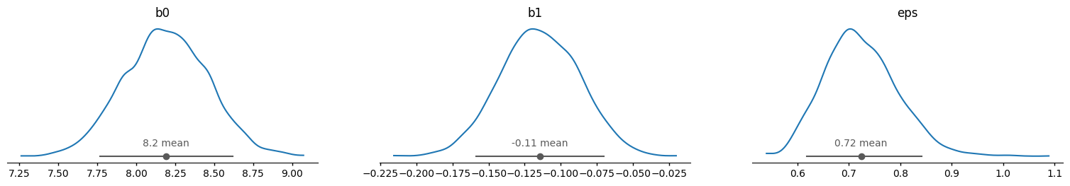

The above plots are the output for our model… I can’t stress this enough! The entire point of using PyMC is to obtain a distribution over model parameters (and predictions), rather than just point estimates. So, when someone asks you to provide “the” output/results of your model, the correct thing to show them is the above plot(s)!

However, if someone is annoyed by that, and wants a “statsmodels-style” output, then as a last resort you can begrudgingly provide them with point estimates and some indicators of uncertainty by calling az.summary():

az.summary(idata.posterior, var_names=['b0', 'b1', 'eps'])

	mean	sd	eti89_lb	eti89_ub	ess_bulk	ess_tail	r_hat	mcse_mean	mcse_sd
b0	8.19	0.268	7.8	8.6	1546	1546	1.00	0.0068	0.0046
b1	-0.115	0.0274	-0.16	-0.07	1524	1488	1.00	0.0007	0.00048
eps	0.724	0.071	0.62	0.84	1890	1980	1.00	0.0016	0.0013

Just please keep in mind how, this is collapsing three entire distributions (plotted above) down into just a box containing a few numbers… Without the full distributions, you will be left with no way to carry out any of the methods we’ll learn in the second half of the course, like e.g. sensitivity analysis: having the full information about uncertainty for each parameter is exactly how we will be able to carry out this kind of “how bad would it be if I’m wrong?” analysis!

b0_mean = float(idata.posterior['b0'].mean())
b1_mean = float(idata.posterior['b1'].mean())
b0_mean, b1_mean

(8.192776586435606, -0.11480798845598969)

az.plot_forest(idata.posterior.mean('chain'), var_names=['b0', 'b1', 'eps']);
plt.show()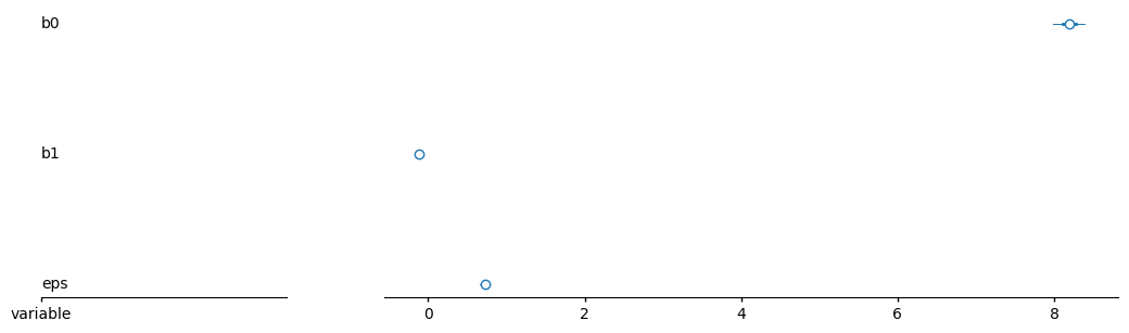

display(idata.posterior['b0'].quantile((.025, .975), dim=("chain", "draw")))
display(idata.posterior['b1'].quantile((.025, .975), dim=("chain", "draw")))

<xarray.DataArray 'b0' (quantile: 2)> Size: 16B
array([7.65930969, 8.71088116])
Coordinates:
  * quantile  (quantile) float64 16B 0.025 0.975

xarray.DataArray

'b0'

• quantile: 2

• 7.659 8.711

  array([7.65930969, 8.71088116])

• Coordinates: (1)
  • quantile
    (quantile)
    float64
    0.025 0.975

    array([0.025, 0.975])

<xarray.DataArray 'b1' (quantile: 2)> Size: 16B
array([-0.167065  , -0.06052311])
Coordinates:
  * quantile  (quantile) float64 16B 0.025 0.975

xarray.DataArray

'b1'

• quantile: 2

• -0.1671 -0.06052

  array([-0.167065  , -0.06052311])

• Coordinates: (1)
  • quantile
    (quantile)
    float64
    0.025 0.975

    array([0.025, 0.975])

post = az.extract(idata.posterior, num_samples=30)
x_plot = xr.DataArray(
  np.linspace(
    country_df['ln_export_pop'].min(),
    country_df['ln_export_pop'].max(),
    100
  ),
  dims="plot_id"
)
lines = post["b0"] + post["b1"] * x_plot
lines2 = b0_mean + b1_mean * x_plot

sns.lmplot(
  x='ln_export_pop', y='ln_maddison_pcgdp2000',
  data=country_df
);
plt.scatter(country_df['ln_export_pop'], country_df['ln_maddison_pcgdp2000'], label="data")
plt.plot(x_plot, lines.transpose(), alpha=0.4, color="C1")
plt.plot(x_plot, lines2.transpose(), alpha=0.9, color='C2')
plt.title("Posterior predictive for normal likelihood");
plt.show()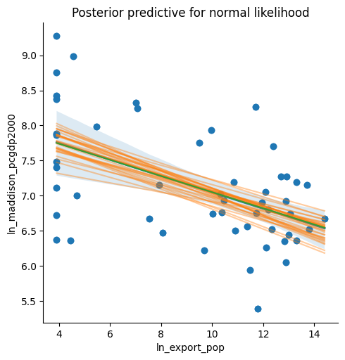

2 Prior Checks

How did we decide what prior to choose? The answer is… very carefully! Let’s look at the impact of our choice of priors on the resulting posterior distributions

with gdp_model:
  idata_pr = pm.sample_prior_predictive(draws=300)

Sampling: [b0, b1, eps, ln_gdp]

_, ax = plt.subplots()

x = xr.DataArray(
  np.linspace(country_df['ln_export_pop'].min(), country_df['ln_export_pop'].max(), 50),
  dims=["plot_dim"]
)
y = idata_pr.prior["b0"] + idata_pr.prior["b1"] * x

ax.plot(x, y.stack(sample=("chain", "draw")), c="k", alpha=0.1)

ax.set_xlabel("Log Slave Exports per Population")
ax.set_ylabel("Log GDP in 2000")
ax.set_title("Prior predictive checks");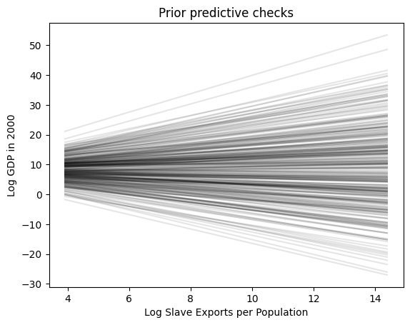

This brings up something a bit… subtle but important about how you can start thinking in a PyMC way rather than an… R or Statsmodels way (though in R, you can use Stan or Ulam instead of PyMC! So if you are an R aficionado, this would be “thinking in a Stan rather than lm way”): since we are learning a language that will allow us to parameterize our models however we’d like, we can think of how we might customize this setup to help us in our modeling task: in other words, having the model “work for us” rather than trying to adapt our thinking to the model!

Specifically, what I’m referring to here is the fact that choosing a prior for \(\beta_0\) means specifying an “initial guess” (plus an uncertainty about that initial guess) for a country with exactly one slave exported (since \(\ln(x) = 0 \iff x = 1\)). Think about how this might be a strange “though experiment” for a researcher trying to understand the impact of slave exports on GDP: they may have expertise on essentially the trajectory of the “average” African country’s history from the era of the Atlantic Slave Trade to the present… and yet in statsmodels, by forcing them to model the intercept here, forces them to have to model a case that is by definition the most extreme possible outlier (since number of slaves exported can’t be less than 1 given the model setup).

And, it gets worse! Those of you who have studied house prices, for example, may have had to estimate a regression modeling how the square footage of a house impacts its price. Modeling the intercept in that case means trying to imagine what a house with 0 square feet might sell for on the housing market…

To avoid this, let’s now just make a slight modification to our PyMC model from above to enable us to do what is much more natural for us as social-scientific modelers: modeling the average or “most typical” unit of observation!

3 Posterior Predictive Checks

with gdp_model:
  pm.sample_posterior_predictive(idata, extend_inferencedata=True)

Sampling: [ln_gdp]

idata.posterior

<xarray.DataTree 'posterior'>
Group: /posterior
    Dimensions:   (chain: 4, draw: 1000, country: 52)
    Coordinates:
      * chain     (chain) int64 32B 0 1 2 3
      * draw      (draw) int64 8kB 0 1 2 3 4 5 6 7 ... 993 994 995 996 997 998 999
      * country   (country) int64 416B 0 1 2 3 4 5 6 7 8 ... 44 45 46 47 48 49 50 51
    Data variables:
        b0        (chain, draw) float64 32kB 8.4 8.27 8.112 ... 8.309 8.304 7.973
        b1        (chain, draw) float64 32kB -0.1311 -0.1293 ... -0.1318 -0.08817
        eps       (chain, draw) float64 32kB 0.7218 0.7429 0.776 ... 0.8215 0.6326
        mean_gdp  (chain, draw, country) float64 2MB 6.512 7.817 ... 7.012 7.274
    Attributes:
        created_at:                 2026-06-19T19:38:08.574493+00:00
        creation_library:           ArviZ
        creation_library_version:   1.1.0
        creation_library_language:  Python
        inference_library:          pymc
        inference_library_version:  6.0.0
        sample_dims:                ['chain', 'draw']
        sampling_time:              1.5081031322479248
        tuning_steps:               1000

xarray.DataTree

'posterior'

• Dimensions:
  • chain: 4
  • draw: 1000
  • country: 52
• Coordinates: (3)
  • chain
    (chain)
    int64
    0 1 2 3

    array([0, 1, 2, 3])

  • draw
    (draw)
    int64
    0 1 2 3 4 5 ... 995 996 997 998 999

    array([  0,   1,   2, ..., 997, 998, 999], shape=(1000,))

  • country
    (country)
    int64
    0 1 2 3 4 5 6 ... 46 47 48 49 50 51

    array([ 0,  1,  2,  3,  4,  5,  6,  7,  8,  9, 10, 11, 12, 13, 14, 15, 16, 17,
           18, 19, 20, 21, 22, 23, 24, 25, 26, 27, 28, 29, 30, 31, 32, 33, 34, 35,
           36, 37, 38, 39, 40, 41, 42, 43, 44, 45, 46, 47, 48, 49, 50, 51])

• Data variables: (4)
  • b0
    (chain, draw)
    float64
    8.4 8.27 8.112 ... 8.304 7.973

    array([[8.40023812, 8.27046346, 8.11233664, ..., 8.0313935 , 8.40200089,
            8.40200089],
           [7.96060093, 7.74324909, 7.84682574, ..., 8.74832929, 8.12331117,
            8.22733068],
           [8.37507531, 8.05832108, 8.18540621, ..., 8.36074117, 7.93747469,
            8.15073276],
           [7.65315441, 7.88951754, 8.42087763, ..., 8.30892363, 8.30445246,
            7.97252957]], shape=(4, 1000))

  • b1
    (chain, draw)
    float64
    -0.1311 -0.1293 ... -0.08817

    array([[-0.13111645, -0.12926183, -0.10698746, ..., -0.10255795,
            -0.1314555 , -0.1314555 ],
           [-0.09340519, -0.06756611, -0.06702613, ..., -0.16949618,
            -0.10982377, -0.11535649],
           [-0.11846937, -0.08570502, -0.12278533, ..., -0.12103874,
            -0.1069809 , -0.10882582],
           [-0.07132009, -0.06719371, -0.11993231, ..., -0.13766112,
            -0.1317926 , -0.08817225]], shape=(4, 1000))

  • eps
    (chain, draw)
    float64
    0.7218 0.7429 ... 0.8215 0.6326

    array([[0.72183697, 0.74286898, 0.77595717, ..., 0.72604419, 0.60574124,
            0.60574124],
           [0.79490697, 0.67518124, 0.6985198 , ..., 0.73600278, 0.65158217,
            0.71429548],
           [0.70674885, 1.06096522, 0.75153672, ..., 0.6888928 , 0.86643758,
            0.82751732],
           [0.68716359, 0.71988528, 0.75558968, ..., 0.74806515, 0.8214549 ,
            0.63257321]], shape=(4, 1000))

  • mean_gdp
    (chain, draw, country)
    float64
    6.512 7.817 6.655 ... 7.012 7.274

    array([[[6.51225953, 7.81655254, 6.65521312, ..., 6.85713708,
             6.97198602, 7.36113789],
            [6.40919012, 7.69503405, 6.55012165, ..., 6.74918942,
             6.86241383, 7.24606119],
            [6.57179746, 7.63606509, 6.68844371, ..., 6.85320816,
             6.94692177, 7.26445912],
            ...,
            [6.55463592, 7.5748406 , 6.66645276, ..., 6.82439562,
             6.91422929, 7.21861991],
            [6.50914022, 7.81680597, 6.65246347, ..., 6.85490958,
             6.9700555 , 7.36021368],
            [6.50914022, 7.81680597, 6.65246347, ..., 6.85490958,
             6.9700555 , 7.36021368]],
    
           [[6.61563619, 7.54479297, 6.71747397, ..., 6.86132126,
             6.94313774, 7.2203631 ],
            [6.77034779, 7.44246789, 6.84401374, ..., 6.94806793,
             7.00725116, 7.20778647],
            [6.88169972, 7.54844834, 6.95477694, ..., 7.05799955,
             7.1167098 , 7.31564245],
    ...
            [6.61787405, 7.82191811, 6.74984012, ..., 6.93624405,
             7.04226561, 7.40150698],
            [6.39702996, 7.46123233, 6.51366905, ..., 6.67842341,
             6.77213127, 7.08964915],
            [6.58372252, 7.66627744, 6.70237309, ..., 6.86996869,
             6.96529258, 7.28828617]],
    
           [[6.62619857, 7.33566177, 6.70395741, ..., 6.81379287,
             6.87626433, 7.08794141],
            [6.92197845, 7.59039412, 6.99523838, ..., 7.09871907,
             7.15757612, 7.35700616],
            [6.69394226, 7.88698002, 6.82470201, ..., 7.009402  ,
             7.11445441, 7.47041191],
            ...,
            [6.32670677, 7.69610345, 6.47679587, ..., 6.68879885,
             6.80938046, 7.21795681],
            [6.40673784, 7.7177569 , 6.55042862, ..., 6.75339388,
             6.86883507, 7.25999374],
            [6.70291532, 7.58001689, 6.79904772, ..., 6.93483609,
             7.01206888, 7.27376293]]], shape=(4, 1000, 52))

• Attributes: (9)

  created_at :

  2026-06-19T19:38:08.574493+00:00

  creation_library :

  ArviZ

  creation_library_version :

  1.1.0

  creation_library_language :

  Python

  inference_library :

  pymc

  inference_library_version :

  6.0.0

  sample_dims :

  ['chain', 'draw']

  sampling_time :

  1.5081031322479248

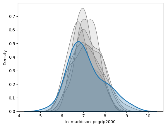
  tuning_steps :

  1000

az.plot_ppc_dist(idata, num_samples=50, kind='kde');
plt.show()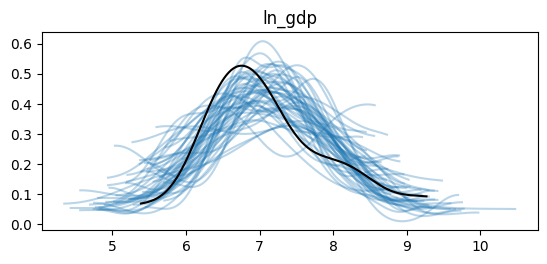

post_pred_draws = idata.posterior_predictive['ln_gdp'].mean('chain')

for cur_draw in post_pred_draws[:6]:
  sns.kdeplot(
    cur_draw,
    fill=True, alpha=0.15, color='grey'
  );
sns.kdeplot(country_df['ln_maddison_pcgdp2000'], fill=True, linewidth=2);
plt.show()