Workshop Week 4: Introduction to PyMC

DSAN 5650: Causal Inference for Computational Social Science
Summer 2026, Georgetown University

Class Sessions

Author

Affiliation

Jeff Jacobs

jj1088@georgetown.edu

Published

Friday, June 12, 2026

DSAN 5650 Workshop 4: Introduction to PyMC

In lecture this week we started by looking at the following PGM, which “lays out” in explicit form many of the implicit assumptions that R’s lm() or Python’s statsmodels.ols() make when you as it to carry out a regression – so, what better way to start learning PyMC than to open it up and start learning how to “re-implement” standard linear regression, but now within a full modeling language that will then allow you to change any parameters you’d like!

And, one benefit of having a custom Coding Workshop just for this class is that, we can also choose a dataset that will help you get comfortable with Computational Social Science while you learn PyMC :) Specifically, we’ll be using a dataset from Nunn and Wantchekon (2011), “The Slave Trade and the Origins of Mistrust in Africa”, which is interesting on its own terms but also gives us an introduction to the Afrobarometer dataset that you’ll be diving into for HW2.

1 Loading the Data

Code

import pandas as pd
import numpy as np

import matplotlib.pyplot as plt
import seaborn as sns

import statsmodels.api as sm
import statsmodels.formula.api as smf

import pymc as pm
import arviz as az
import xarray as xr
import preliz as pz

Code

nunn_data_url = "https://github.com/jpowerj/dsan-content/raw/refs/heads/main/2026-sum-dsan5650/workshop01/slave_trade_QJE.dta"
country_df = pd.read_stata(nunn_data_url)
country_df.head()

	isocode	country	ln_maddison_pcgdp2000	ln_export_area	ln_export_pop	colony1	colony2	colony3	colony4	...	ln_avg_oil_pop	ln_avg_all_diamonds_pop	ln_pop_dens_1400	atlantic_distance_minimum	indian_distance_minimum	saharan_distance_minimum	red_sea_distance_minimum	ethnic_fractionalization	state_dev	land_area
0	AGO	Angola	6.670766	7.967494	14.399250	0.0	0.0	1.0	0.0	...	0.643126	-1.701396	-0.024917	5.668760	6.980571	4.925892	3.872354	0.7867	0.635	1.2500
1	BDI	Burundi	6.354370	1.140843	4.451658	0.0	0.0	0.0	1.0	...	-9.210340	-6.907755	3.036856	10.626214	2.570375	3.718742	2.215324	0.2951	0.995	0.0278
2	BEN	Benin	7.187657	8.304137	13.308970	0.0	1.0	0.0	0.0	...	-3.531555	-6.907755	1.214196	5.120652	9.233961	2.834785	3.901736	0.7872	0.695	0.1130
3	BFA	Burkina Faso	6.748760	6.413822	11.724286	0.0	1.0	0.0	0.0	...	-9.210340	-6.907755	0.908565	4.774938	9.299419	2.763519	4.239375	0.7377	0.338	0.2740
4	BWA	Botswana	8.377471	-2.302585	3.912023	1.0	0.0	0.0	0.0	...	-9.210340	2.186849	-2.075029	5.686335	5.764575	5.856533	4.299600	0.4102	0.893	0.6000

5 rows × 39 columns

Code

country_df.columns

Index(['isocode', 'country', 'ln_maddison_pcgdp2000', 'ln_export_area',
       'ln_export_pop', 'colony0', 'colony1', 'colony2', 'colony3', 'colony4',
       'colony5', 'colony6', 'colony7', 'abs_latitude', 'longitude',
       'rain_min', 'humid_max', 'low_temp', 'ln_coastline_area', 'island_dum',
       'islam', 'legor_fr', 'legor_uk', 'region_n', 'region_s', 'region_w',
       'region_e', 'region_c', 'ln_avg_gold_pop', 'ln_avg_oil_pop',
       'ln_avg_all_diamonds_pop', 'ln_pop_dens_1400',
       'atlantic_distance_minimum', 'indian_distance_minimum',
       'saharan_distance_minimum', 'red_sea_distance_minimum',
       'ethnic_fractionalization', 'state_dev', 'land_area'],
      dtype='str')

2 “Off-the-Shelf” Regression with `statsmodels`

Code

sns.lmplot(
  x='ln_export_pop', y='ln_maddison_pcgdp2000',
  data=country_df
);
plt.show()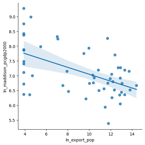

Code

gdp_model_sm = smf.ols('ln_maddison_pcgdp2000 ~ ln_export_pop', data=country_df).fit()
gdp_model_sm.summary()

OLS Regression Results
Dep. Variable:	ln_maddison_pcgdp2000	R-squared:	0.271
Model:	OLS	Adj. R-squared:	0.257
Method:	Least Squares	F-statistic:	18.62
Date:	Fri, 12 Jun 2026	Prob (F-statistic):	7.52e-05
Time:	19:01:34	Log-Likelihood:	-55.065
No. Observations:	52	AIC:	114.1
Df Residuals:	50	BIC:	118.0
Df Model:	1
Covariance Type:	nonrobust

	coef	std err	t	P>\|t\|	[0.025	0.975]
Intercept	8.2151	0.269	30.499	0.000	7.674	8.756
ln_export_pop	-0.1168	0.027	-4.315	0.000	-0.171	-0.062

Omnibus:	0.176	Durbin-Watson:	2.527
Prob(Omnibus):	0.916	Jarque-Bera (JB):	0.376
Skew:	0.058	Prob(JB):	0.829
Kurtosis:	2.600	Cond. No.	27.4

Notes:
[1] Standard Errors assume that the covariance matrix of the errors is correctly specified.

2.1 What Do We Get? …A Point Estimate of the Mean, and a Point Estimate of Uncertainty

Code

# 3. Plot coefficients and 95% Confidence Intervals
param_df = gdp_model_sm.params.reset_index()
param_df.columns = ['Feature', 'Coefficient']
param_df = param_df.set_index('Feature')
# display(param_df)
conf_df = gdp_model_sm.conf_int()
conf_df.columns = ['Lower_CI', 'Upper_CI']
# display(conf_df)

full_coef_df = pd.concat([param_df, conf_df], axis=1).reset_index() \
  .rename(columns={'index': 'Feature'})
display(full_coef_df)

def plot_coefs(coef_df):
  plt.figure(figsize=(8, 1))
  sns.pointplot(
    data=coef_df, 
    x='Coefficient', 
    y='Feature',
    linestyle='none',
    errorbar=None,
    markers='o', 
    color='black'
  )
  # Manually add confidence intervals
  for idx, row in coef_df.reset_index().iterrows():
    plt.plot(
      [row['Lower_CI'], row['Upper_CI']], 
      [idx, idx], 
      color='black', 
      linewidth=2
    )
  # Vertical line representing 0 (no effect)
  plt.axvline(0, color='gray', linestyle='--', linewidth=1)
  plt.title('Regression Coefficients and 95% Confidence Intervals')
  plt.show()

# Plot intercept
plot_coefs(full_coef_df[full_coef_df['Feature'] == 'Intercept'])
# Plot effect
b1_df = full_coef_df[full_coef_df['Feature'] == 'ln_export_pop'].copy()
plot_coefs(b1_df)

	Feature	Coefficient	Lower_CI	Upper_CI
0	Intercept	8.215094	7.674079	8.756109
1	ln_export_pop	-0.116754	-0.171097	-0.062410

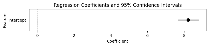
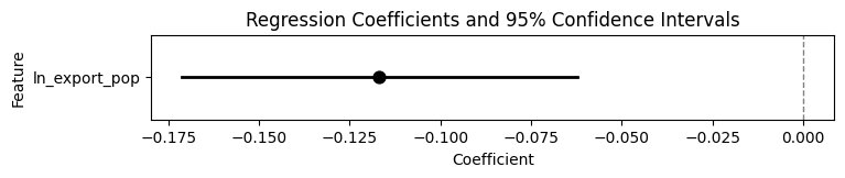
I know it’s difficult if your brain has been trained to think that this is “the” information you can learn about the world from a regression, but try to think of the underlying scenarios that might be “masked” by the fact that we can only view a single point estimate (the dot) and a single uncertainty estimate (the width of the lines on either side of the dot). For example: is -0.117 actually the “most likely” value of the coefficient? Or, could this arise from a case where there are two “humps” in our distribution, at (say) -0.1 and -0.14, that “average out” to -0.117…

Another issue is… less mathematical and more interpretive, but also maybe more important: from your introductory stats class onwards, you have to constantly be reminded that a 95% confidence interval does not mean an interval with 95% probability of containing the true value! Instead, you have to constantly tamp down your intuition, and remember some strange statement about how “if you repeated the sampling procedure infinitely many times, 95% of those times the resulting interval would contain this parameter value”. Well, bucko, get excited because you won’t need to do that anymore with a Bayesian model like the ones you’ll be implementing here in PyMC!

By explicitly placing a prior probability on each parameter, you obtain a natural/intuitive implicational statement: “Given this prior, in combination with the data, there is a 95% chance that the true value is between \(x\) and \(y\)”

With the powerful computational tools we have at our disposal (multicore processors, parallelization, neural networks, etc.), we don’t have to “settle” for just two pieces of information about the intercept and the effect of slave exports, and we don’t have to “settle” for the default “flat priors” that then require weird statements about infinitely repeating sampling procedures. We can use these tools to estimate the full distribution of our uncertainty about these values, which is exactly what PyMC enables, by keeping full mathematical representations of both our prior knowledge (our distribution of likely parameter values before looking at the data) and posterior knowledge (our distribution of likely parameter values after looking at the data).

4 “Customizable” Regression with PyMC

Code

import pymc as pm

gdp_coords = {
  'country': list(range(len(country_df))),
}
print(gdp_coords)

{'country': [0, 1, 2, 3, 4, 5, 6, 7, 8, 9, 10, 11, 12, 13, 14, 15, 16, 17, 18, 19, 20, 21, 22, 23, 24, 25, 26, 27, 28, 29, 30, 31, 32, 33, 34, 35, 36, 37, 38, 39, 40, 41, 42, 43, 44, 45, 46, 47, 48, 49, 50, 51]}

Code

with pm.Model(coords=gdp_coords) as gdp_model:
  # Observed Data
  slave_exports_obs = pm.Data(
    "slave_exports_obs",
    country_df['ln_export_pop'],
    dims='country',
  )
  ln_gdp_obs = pm.Data(
    "ln_gdp_obs",
    country_df['ln_maddison_pcgdp2000'],
    dims='country',
  )
  # X, Y nodes set up in PyMC

  # Parameters
  b0 = pm.Normal('b0', mu=8, sigma=0.5)
  b1 = pm.Normal('b1', mu=0, sigma=0.5)
  eps = pm.HalfNormal('eps', sigma=4)

  # Linking them together!
  mean_ln_gdp = pm.Deterministic(
    'mean_gdp',
    b0 + b1 * slave_exports_obs,
    dims='country',
  )
  ln_gdp = pm.Normal(
    'ln_gdp',
    mu=mean_ln_gdp, sigma=eps,
    observed=ln_gdp_obs,
    dims='country',
  )

gdp_model.to_graphviz()

Code

with gdp_model:
  idata = pm.sample(num_draws=1000)

Initializing NUTS using jitter+adapt_diag...
Multiprocess sampling (4 chains in 4 jobs)
NUTS: [b0, b1, eps]

Sampling 4 chains for 1_000 tune and 1_000 draw iterations (4_000 + 4_000 draws total) took 2 seconds.

Code

idata

Code

az.plot_dist(
  idata.posterior,
  var_names=['b0','b1', 'eps'],
);
plt.show()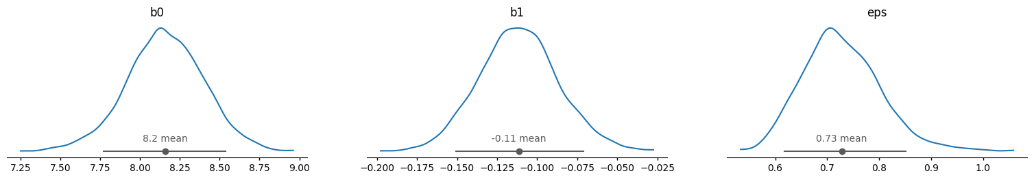

Code

b0_mean = float(idata.posterior['b0'].mean())
b1_mean = float(idata.posterior['b1'].mean())
b0_mean, b1_mean

(8.161833487707938, -0.11172543274908432)

Code

az.summary(idata.posterior, var_names=['b0', 'b1', 'eps'])

	mean	sd	eti89_lb	eti89_ub	ess_bulk	ess_tail	r_hat	mcse_mean	mcse_sd
b0	8.16	0.237	7.8	8.5	1447	1666	1.00	0.0063	0.0047
b1	-0.112	0.024	-0.15	-0.073	1466	1672	1.00	0.00064	0.0005
eps	0.724	0.075	0.62	0.85	2043	1992	1.00	0.0017	0.0014

Code

az.plot_forest(idata.posterior.mean('chain'), var_names=['b0', 'b1']);
plt.show()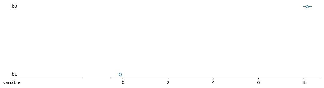

Code

print(idata.posterior['b0'].quantile((.025, .975), dim=("chain", "draw")))
print(idata.posterior['b1'].quantile((.025, .975), dim=("chain", "draw")))

<xarray.DataArray 'b0' (quantile: 2)> Size: 16B
array([7.68464826, 8.61926868])
Coordinates:
  * quantile  (quantile) float64 16B 0.025 0.975
<xarray.DataArray 'b1' (quantile: 2)> Size: 16B
array([-0.15813826, -0.06430003])
Coordinates:
  * quantile  (quantile) float64 16B 0.025 0.975

Code

post = az.extract(idata.posterior, num_samples=30)
x_plot = xr.DataArray(
  np.linspace(
    country_df['ln_export_pop'].min(),
    country_df['ln_export_pop'].max(),
    100
  ),
  dims="plot_id"
)
lines = post["b0"] + post["b1"] * x_plot
lines2 = b0_mean + b1_mean * x_plot

sns.lmplot(
  x='ln_export_pop', y='ln_maddison_pcgdp2000',
  data=country_df
);
plt.scatter(country_df['ln_export_pop'], country_df['ln_maddison_pcgdp2000'], label="data")
plt.plot(x_plot, lines.transpose(), alpha=0.4, color="C1")
plt.plot(x_plot, lines2.transpose(), alpha=0.9, color='C2')
plt.title("Posterior predictive for normal likelihood");
plt.show()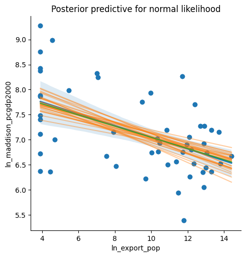

4 Prior Checks

How tf did we decide what prior to choose? The answer is… very carefully! Let’s bring in PreliZ

Code

with gdp_model:
  idata_pr = pm.sample_prior_predictive(draws=300)

Sampling: [b0, b1, eps, ln_gdp]

Code

_, ax = plt.subplots()

x = xr.DataArray(
  np.linspace(country_df['ln_export_pop'].min(), country_df['ln_export_pop'].max(), 50),
  dims=["plot_dim"]
)
y = idata_pr.prior["b0"] + idata_pr.prior["b1"] * x

ax.plot(x, y.stack(sample=("chain", "draw")), c="k", alpha=0.1)

ax.set_xlabel("Log Slave Exports per Population")
ax.set_ylabel("Log GDP in 2000")
ax.set_title("Prior predictive checks");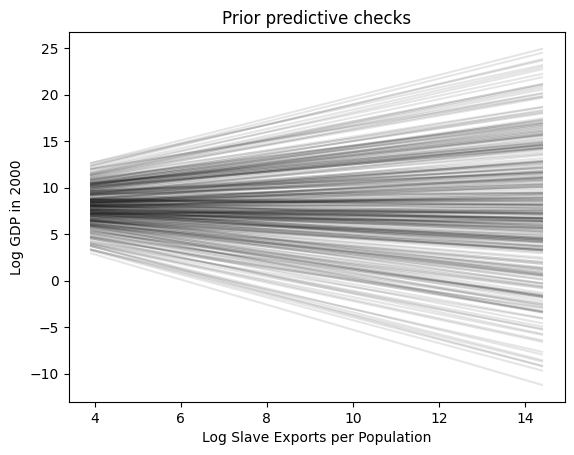

This brings up something a bit… subtle but important about how you can start thinking in a PyMC way rather than an… R or Statsmodels way (though in R, you can use Stan or Ulam instead of PyMC! So if you are an R aficionado, this would be “thinking in a Stan rather than lm way”): since we are learning a language that will allow us to parameterize our models however we’d like, we can think of how we might customize this setup to help us in our modeling task: in other words, having the model “work for us” rather than trying to adapt our thinking to the model!

Specifically, what I’m referring to here is the fact that choosing a prior for \(\beta_0\) means specifying an “initial guess” (plus an uncertainty about that initial guess) for a country with exactly one slave exported (since \(\ln(x) = 0 \iff x = 1\)). Think about how this might be a strange “though experiment” for a researcher trying to understand the impact of slave exports on GDP: they may have expertise on essentially the trajectory of the “average” African country’s history from the era of the Atlantic Slave Trade to the present… and yet in statsmodels, by forcing them to model the intercept here, forces them to have to model a case that is by definition the most extreme possible outlier (since number of slaves exported can’t be less than 1 given the model setup).

And, it gets worse! Those of you who have studied house prices, for example, may have had to estimate a regression modeling how the square footage of a house impacts its price. Modeling the intercept in that case means trying to imagine what a house with 0 square feet might sell for on the housing market…

To avoid this, let’s now just make a slight modification to our PyMC model from above to enable us to do what is much more natural for us as social-scientific modelers: modeling the average or “most typical” unit of observation!

5 Posterior Predictive Checks

Code

with gdp_model:
  pm.sample_posterior_predictive(idata, extend_inferencedata=True)

Sampling: [ln_gdp]

Code

idata.posterior

Code

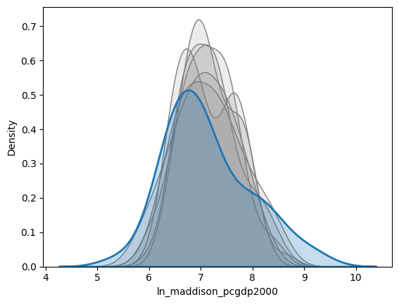
az.plot_ppc_dist(idata, num_samples=50, kind='kde');
plt.show()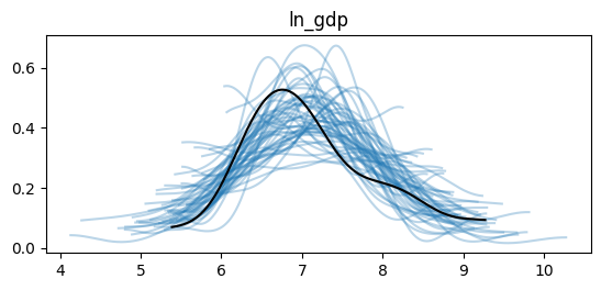

Code

post_pred_draws = idata.posterior_predictive['ln_gdp'].mean('chain')

Code

for cur_draw in post_pred_draws[:6]:
  sns.kdeplot(
    cur_draw,
    fill=True, alpha=0.15, color='grey'
  );
sns.kdeplot(country_df['ln_maddison_pcgdp2000'], fill=True, linewidth=2);
plt.show()

DSAN 5650 Workshop 4: Introduction to PyMC

1 Loading the Data

2 “Off-the-Shelf” Regression with statsmodels

2.1 What Do We Get? …A Point Estimate of the Mean, and a Point Estimate of Uncertainty

4 “Customizable” Regression with PyMC

4 Prior Checks

5 Posterior Predictive Checks

2 “Off-the-Shelf” Regression with `statsmodels`