Week 13: Visualization Tools for Final Projects
PPOL 6805 / DSAN 6750: GIS for Spatial Data Science
Fall 2026
Jeff Jacobs
Wednesday, November 18, 2026
Final Project Details
- Project Showcase: 6:30-9pm, Wed, December 2, 2026
- Come eat falafel and show off your cool visualizations and regression coefficients!
- Reports: Due 5:59pm, Fri, December 11, 2026
- If you’re in DSAN 6000 and you’re worried about that final project… See calendar! (In two slides)
Research Methodology: Hypotheses
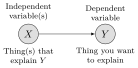
Social Science (McCourt):
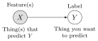
Machine Learning (DSAN):
Due Date Details
Visualizing Spatial Data
- My recommendation for final presentations: Tiptoe from
mapview\leadsto Leaflet!
Code
library(leaflet) |> suppressPackageStartupMessages()
library(leaflet.extras2) |> suppressPackageStartupMessages()
library(mapview) |> suppressPackageStartupMessages()
set.seed(6805)
city_df <- tibble::tribble(
  ~city, ~lon, ~lat, ~pop,
  "Chicago", 41.950567516553896, -87.93011127491978, 2746388,
  "Detroit", 42.45123004999075, -83.18402319217698, 631524
)
city_sf <- sf::st_as_sf(
  city_df,
  coords = c("lat", "lon"),
  # Reminder: CRS 4326 is more *efficient* for web
  # display (uses less memory on average);
  # CRS 3857 is less efficient (uses more memory
  # on average), since it includes info necessary
  # for precise *distance* calculations (hence
  # spatstat's 3857 requirement for ppp objects)
  crs=4326
)
city_buf_sf <- city_sf |> sf::st_buffer(20000)
city_cases_sf <- city_buf_sf |>
  sf::st_sample(size=rep(10,2)) |>
  sf::st_as_sf()
city_cases_sf$city <- "Detroit (10 Cases)"
city_cases_sf[1:10, 'city'] <- "Chicago (10 Cases)"
city_cases_sf$sample <- "Flu"
# Now sample from *population* to visualize
# *base rates*
city_pop_sf <- city_buf_sf |>
  sf::st_sample(size=c(16, 4)) |>
  sf::st_as_sf()
city_pop_sf$city <- "Detroit"
city_pop_sf[1:16, 'city'] <- "Chicago"
city_pop_sf$sample <- "People"
# Uncomment for "plain" mapview output (compare!)
# city_combined_sf <- bind_rows(
#   city_cases_sf,
#   city_pop_sf
# )
# mapview(
#   city_combined_sf, zcol="city", marker="sample"
# )
# Custom icon from *local* image for flu cases
Flu = makeIcon(
    iconUrl="images/Maki2-danger-24.svg",
    iconRetinaUrl="images/Maki2-danger-24.svg",
    iconWidth=20,
    iconHeight=20,
    className='highlight-icon'
)
# Custom icon from *web* image for base rates
People = makeIcon(
  iconUrl="https://upload.wikimedia.org/wikipedia/commons/e/ef/Maki2-pitch-24.svg",
  iconRetinaUrl="https://upload.wikimedia.org/wikipedia/commons/e/ef/Maki2-pitch-24.svg",
  iconWidth=20,
  iconHeight=20
)
leaflet(city_cases_sf) |>
  addProviderTiles("Esri.WorldGrayCanvas") |>
  # addProviderTiles("CartoDB.Positron") |>
  addMarkers(data=city_cases_sf, icon = Flu) |>
  addMarkers(data=city_pop_sf, icon = People) |>
  addControl(
    html_legend(
      urls   = c("https://raw.githubusercontent.com/jpowerj/dsan-content/refs/heads/main/2026-fall-ppol6805/Maki2-danger-24.svg", "https://upload.wikimedia.org/wikipedia/commons/e/ef/Maki2-pitch-24.svg"),
      labels = c("Flu", "At Risk"),
      title  = "Status"
    ),
    position = "bottomright"
  ) |>
  addControl(
    html_label("Chicago<br>Population 2.7 million"),
    position = "topleft"
  ) |>
  addControl(
    html_label("Detroit, MI<br>Population 650,000"),
    position = "topright"
  )
You’ve Secretly Been Using Leaflet All Along!
Setup Code
library(tidyverse) |> suppressPackageStartupMessages()
library(sf) |> suppressPackageStartupMessages()
library(osmdata) |> suppressPackageStartupMessages()
library(mapview) |> suppressPackageStartupMessages()
get_osm_cached <- function(query, cache_file, tries = 3) {
  if (file.exists(cache_file)) {
    message("Loading cached data from ", cache_file)
    return(readRDS(cache_file))
  }
  for (i in seq_len(tries)) {
    result <- tryCatch(
      osmdata_sf(query),
      error = function(e) {
        message("Attempt ", i, " failed: ", conditionMessage(e))
        NULL
      }
    )
    if (!is.null(result)) {
      saveRDS(result, cache_file)
      message("Saved to ", cache_file)
      return(result)
    }
    Sys.sleep(5)
  }
  stop("Failed to fetch after ", tries, " attempts.")
}
nh_bbox <- getbb("New Haven, CT")
highway_result <- opq(bbox=nh_bbox) |>
  add_osm_feature(
    key = "highway",
    value = "motorway"
  )
transport_result <- opq(bbox=nh_bbox) |>
  add_osm_feature(
    key="public_transport"
  )
nh_road_sfs <- get_osm_cached(highway_result, "data/nh_road_sfs.rds")
nh_transport_sfs <- get_osm_cached(transport_result, "data/nh_transport_sfs.rds")
nh_road_sf <- nh_road_sfs$osm_linesPutting Things Into Leaflet
- Let’s go take a look at the Getting GIS Data writeup!
- Constructing “Overpass Queries”:
Application: Urban Segregation
Step : Mapping Inequality

Spatial Data Science
Step Quantifying and evaluating hypotheses about urban segregation
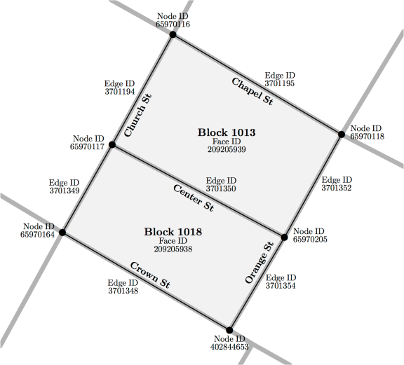
From Roberto and Hwang (2017)
Straight-Line vs. Street Distance
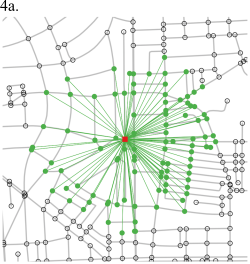
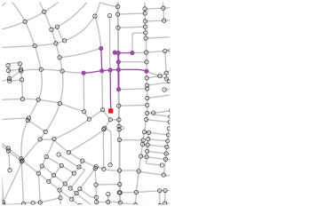
…Evaluating Impacts of Policy Interventions!

Custom Bounding Box
Code
custom_upper_left <- c(41.362432360113566, -72.9722636671877)
custom_lower_right <- c(41.34295668062255, -72.9385289699316)
bbox_coords <- c(
  custom_upper_left[2],
  custom_upper_left[1],
  custom_lower_right[2],
  custom_lower_right[1]
)
names(bbox_coords) = c("xmin","ymin","xmax","ymax")
custom_sf <- st_as_sf(
  st_as_sfc(
    st_bbox(bbox_coords)
  ),
  crs=4326
)
# nh_query <- opq(bbox=bbox_coords) |>
#   add_osm_feature(
#     key = "highway"
#   )
# nh_sfs <- osmdata_sf(nh_query)
# nh_road_sf <- nh_sfs$osm_lines
# mapview(nh_road_sf)
mapview(custom_sf)
References
Massey, Douglas S., and Nancy A. Denton. 1993. American Apartheid: Segregation and the Making of the Underclass. Harvard University Press.
Roberto, Elizabeth, and Jackelyn Hwang. 2017. “Barriers to Integration: Physical Boundaries and the Spatial Structure of Residential Segregation.”
PPOL 6805 Week 13: Visualization