Week 10: Evaluating Spatial Hypotheses II: Base Rates and Null Models

PPOL 6805 / DSAN 6750: GIS for Spatial Data Science
Fall 2026

Jeff Jacobs

jj1088@georgetown.edu

Wednesday, October 28, 2026

Roadmap to the Midterm!

✅ Last Week (Oct 21): Framework for Formalizing Point \leadsto Areal Hypotheses

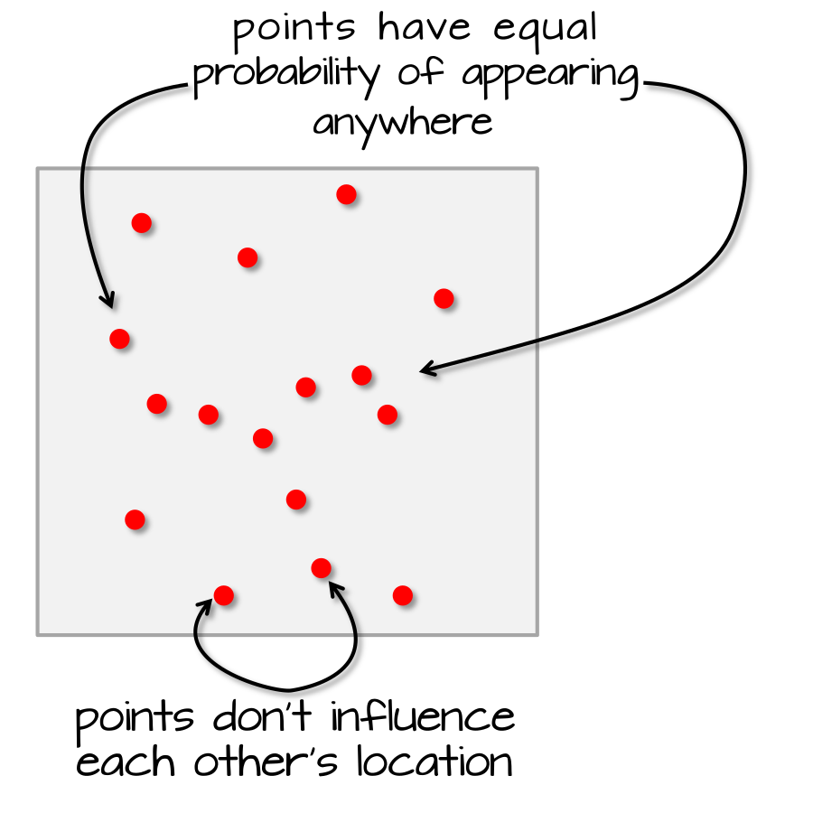
Repulsion ← Complete Spatial Randomness → Clustering
  • 🔲 Today (Oct 28): Using this framework to Evaluate Point \leadsto Areal Hypotheses
  • 🔲 Midterm (Nov 4): “Mini-homework” on Spatial Data Science unit (same topics as HW2-3)!

Where We Left Off: The Tree-Grid Mystery

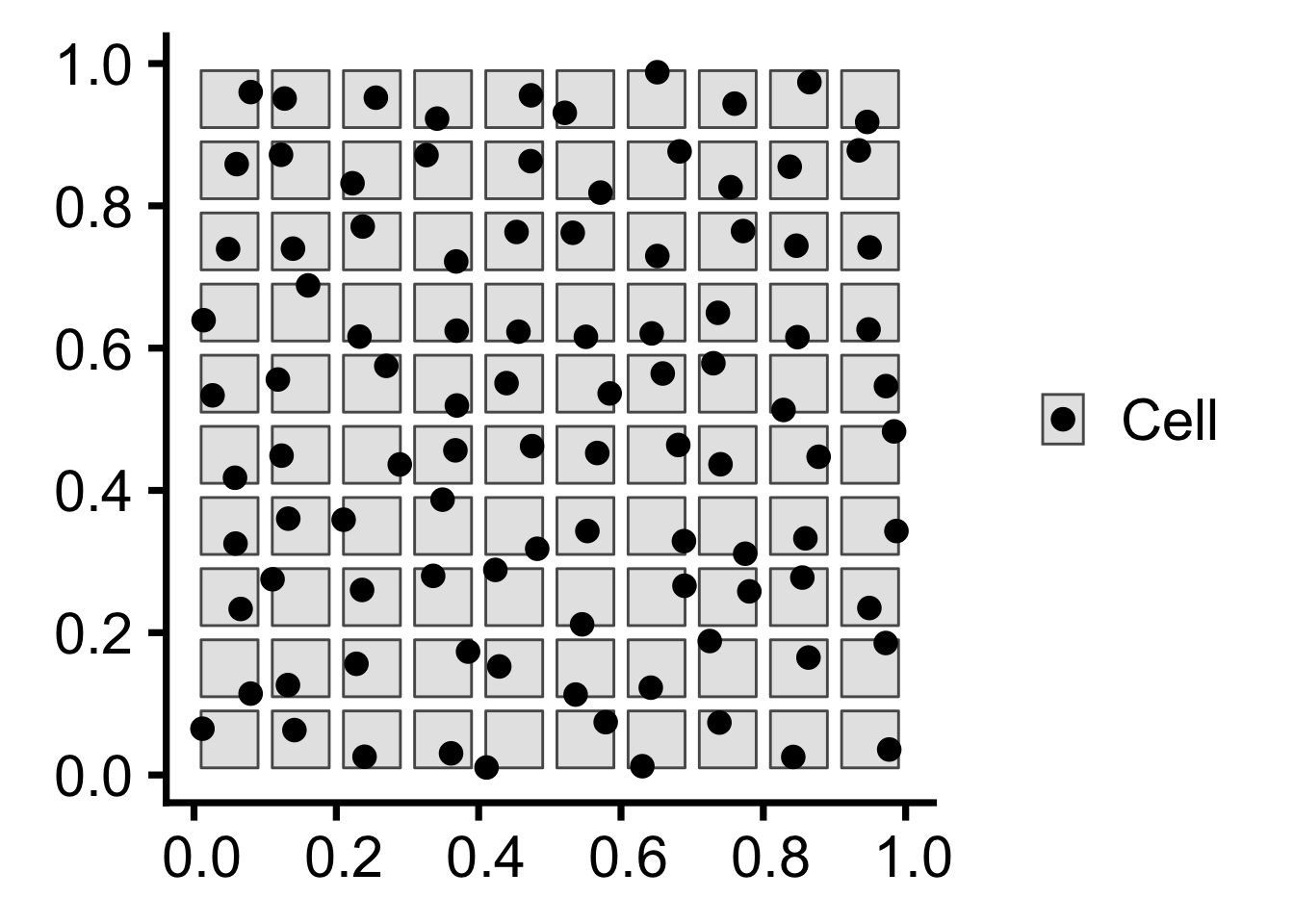
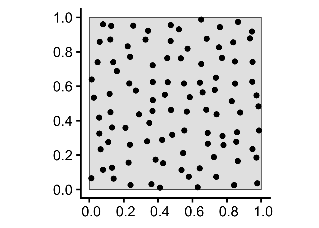
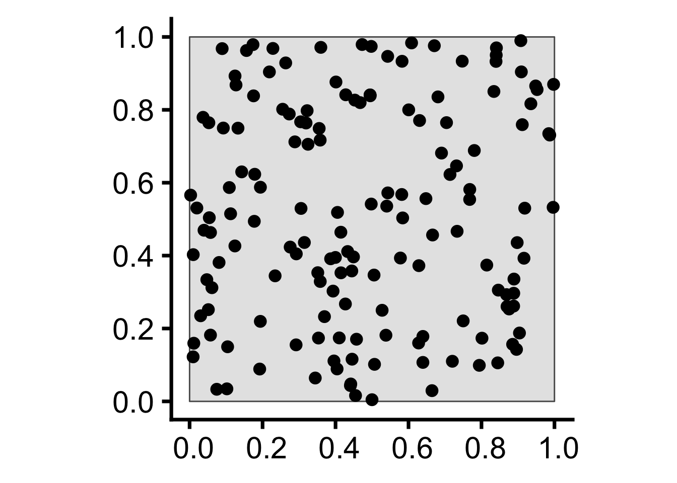
You’ve been hired as an archaeologist – congratulations! Your job: determine whether arrangement of trees formed:

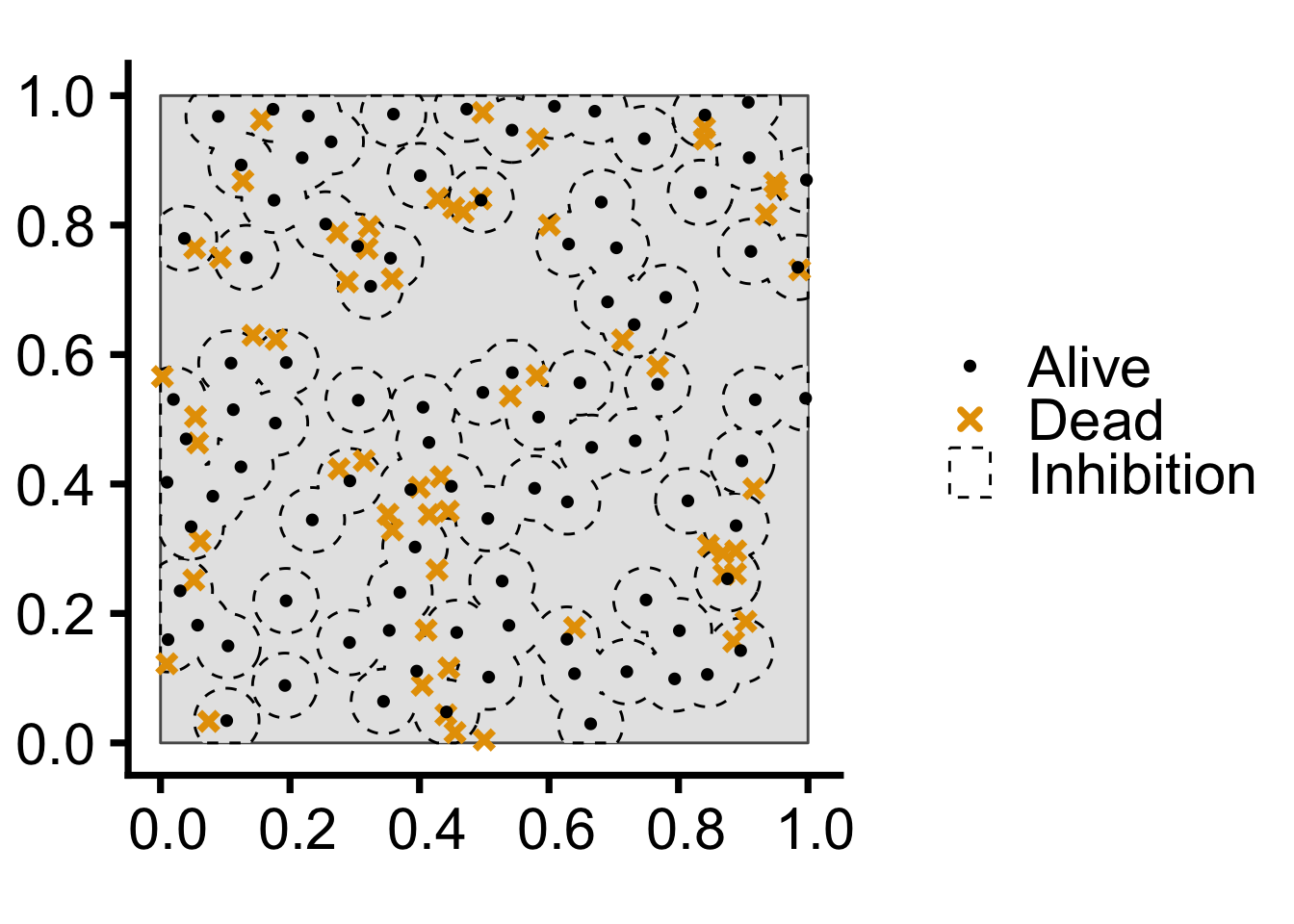
  • Naturally, via a process of resource competition, or
  • Artificially, via an ancient civilization planting in a grid…

Two Possible Histories…

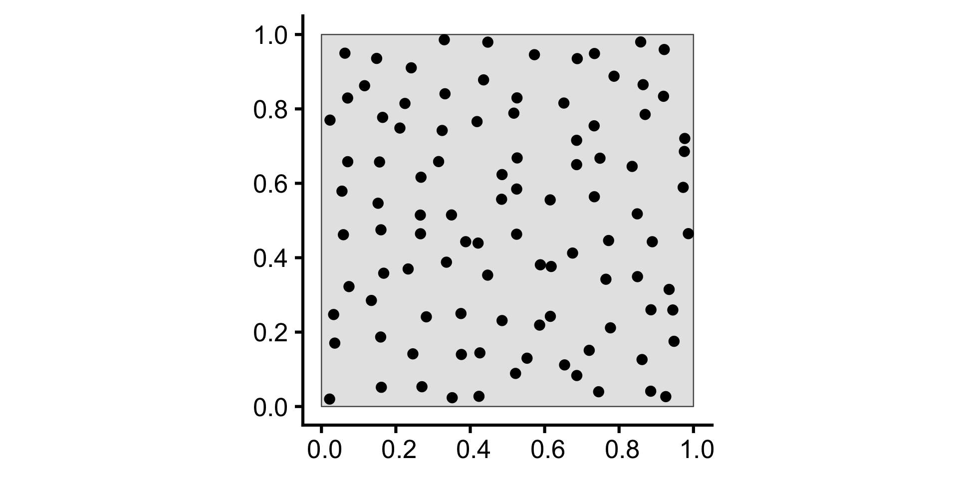
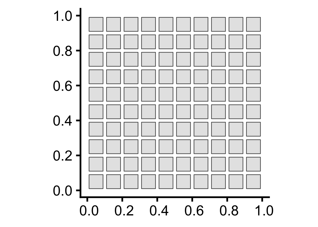
Hypothesis \mathcal{H}_{\textsf{Art}}: Artificial Formation
Code (Step 1: Grid Creation)
ha_base <- 28
square_sf <- sf::st_as_sf(spatstat.geom::square(1))
grid_sf <- sf::st_as_sf(sf::st_make_grid(square_sf))
grid_buffer_sf <- grid_sf |> sf::st_buffer(dist=-0.01, singleSide = TRUE)
grid_buffer_sf |> ggplot() +
  geom_sf() +
  theme_classic(base_size=ha_base) +
  transparent_bg()

Code (Step 2: Point Generation)
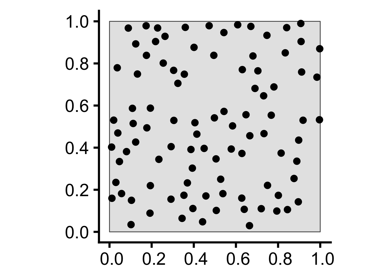
grid_points <- sf::st_sample(grid_buffer_sf, size=rep(1,100))
grid_buffer_sf |> ggplot(aes(shape='Cell')) +
  geom_sf() +
  geom_sf(data=grid_points) +
  scale_shape_manual("Shape", values=c('Cell'=19)) +
  theme_classic(base_size=ha_base) +
  theme(
    legend.title = element_blank(),
    # legend.text = element_text(size=18)
  ) +
    transparent_bg()

Code (Step 3: Observed Result)
grid_ppp <- as.ppp(grid_points, W=spatstat.geom::square(1))
grid_ppp |> sf::st_as_sf() |> ggplot() +
  geom_sf() +
  theme_classic(base_size=ha_base) +
  transparent_bg()

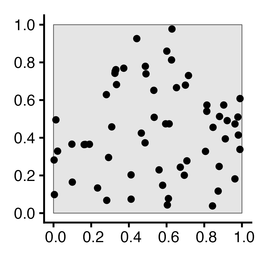
Hypothesis \mathcal{H}_{\textsf{Nat}}: Natural Formation
Code (Step 1: Tree Generation)
hn_base <- 28
r <- 0.05
pois_ppp <- rpoispp(150)
pois_sf <- pois_ppp |> sf::st_as_sf()
pois_sf |> ggplot() +
  geom_sf() +
  theme_classic(base_size=hn_base) +
  transparent_bg()

Code (Step 2: Competition)
age <- runif(npoints(pois_ppp))
pair_dists <- pairdist(pois_ppp)
close <- (pair_dists < r)
later <- outer(age, age, ">")
killed <- apply(close & later, 1, any)
killed_ppp <- pois_ppp[killed]
alive_ppp <- pois_ppp[!killed]
pois_window_sf <- pois_ppp |> sf::st_as_sf() |> filter(label=="window")
pois_killed_sf <- killed_ppp |> sf::st_as_sf() |> filter(label=="point")
pois_alive_sf <- alive_ppp |> sf::st_as_sf() |> filter(label=="point")
alive_buff_sf <- pois_alive_sf |> sf::st_buffer(r) |> sf::st_union() |> sf::st_intersection(pois_window_sf)
ggplot() +
  geom_sf(data=pois_window_sf) +
  geom_sf(data=alive_buff_sf, aes(color='Inhibition', shape='Inhibition'), linetype='dashed') +
  geom_sf(data=pois_killed_sf, aes(color='Dead', shape='Dead'), size=2, stroke=2) +
  geom_sf(data=pois_alive_sf, aes(color='Alive', shape='Alive'), size=1, stroke=1) +
  scale_shape_manual(name=NULL, values=c("Alive"=19, "Dead"=4, 'Inhibition'=21), labels=c("Alive", "Dead", "Inhibition")) +
  scale_color_manual(name=NULL, values=c("Alive"="black", "Dead"=cb_palette[1], "Inhibition"="black"), labels=c("Alive", "Dead", "Inhibition")) +
  guides(shape=guide_legend(override.aes=list(fill = "white"))) +
  theme_classic(base_size = hn_base) +
  theme(plot.margin = unit(c(0,0,0,0), "cm")) +
  transparent_bg()

Code (Step 3: Observed Result)
alive_ppp |> sf::st_as_sf() |> ggplot() +
  geom_sf() +
  theme_classic(base_size=hn_base) +
  transparent_bg()

What Tools Do We Have for Distinguishing Between These Cases?

“First-Order” measures

vs.

“Second-Order” measures

  • Pick any point (“site”) \mathbf{s} on map
  • What is \Pr(Event occurs at \mathbf{s})?
  • Assume already-observed event at \mathbf{s}
  • What is \Pr(Another event nearby \mathbf{s})?

Why Do Events Appear Where They Do?

Code
library(tidyverse)
library(spatstat)
set.seed(6809)
N <- 60
r_core <- 0.05
obs_window <- square(1)
### Clustered data
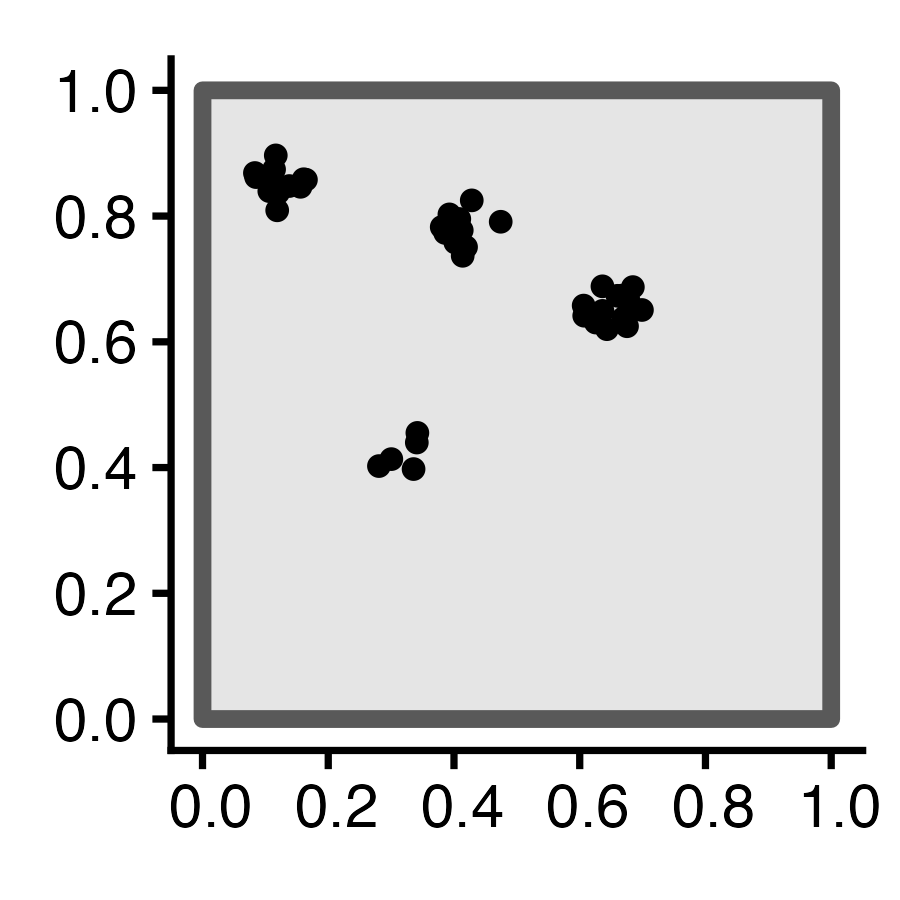
clust_ppp <- rMatClust(
  kappa=6,
  scale=r_core,
  mu=10
)
clust_sf <- clust_ppp |> sf::st_as_sf()
clust_plot <- clust_sf |>
  ggplot() +
  geom_sf(size=2) +
  theme_classic(base_size=18) +
  transparent_bg()
ggsave("images/clust_ppp.png", clust_plot, width=3, height=3)
# Intensity fn
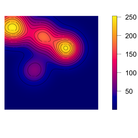
clust_intensity <- density(clust_ppp, sigma = 0.1)
png("images/clust_intensity.png")
par(mar=c(1.5,0,0,2), las=2, oma=c(0,0,0,0), cex=2, bg=NA)
plot(clust_intensity, main=NULL)
contour(clust_intensity, add = TRUE)
dev.off()
### PCF
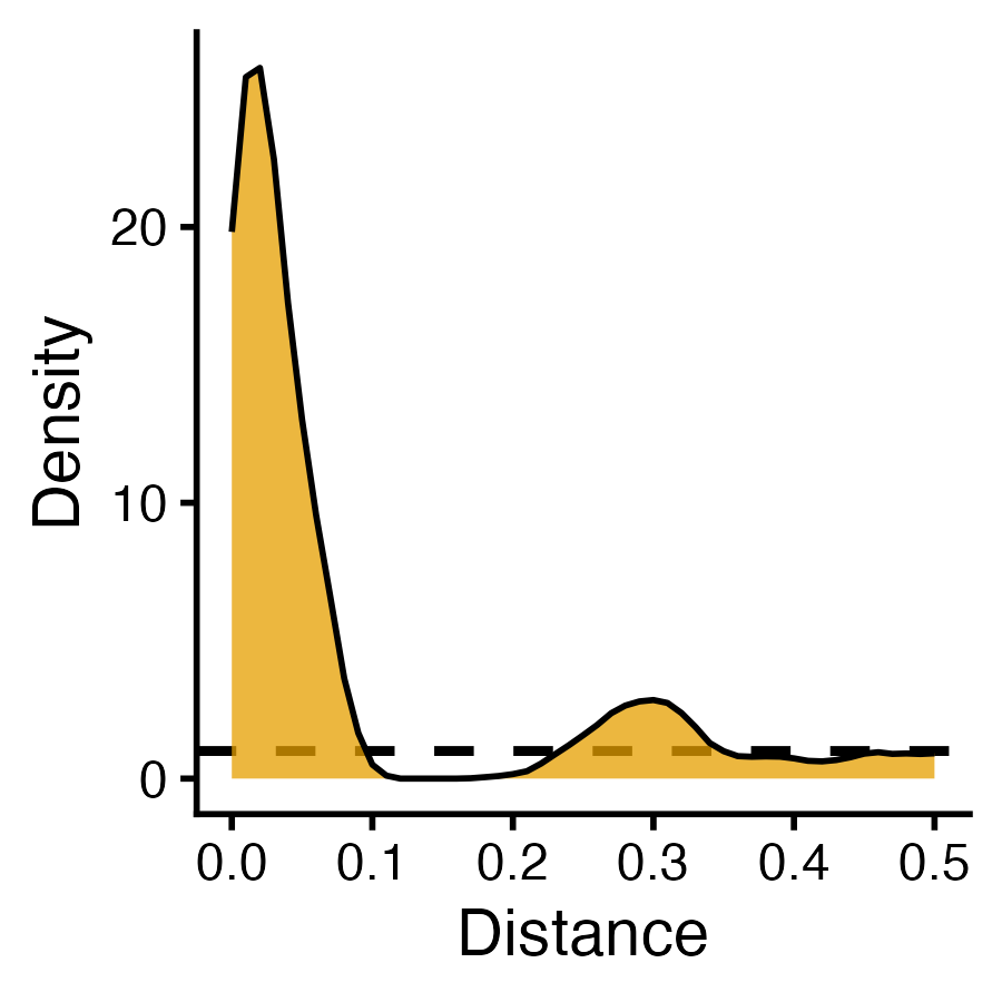
clust_pcf <- spatstat.explore::pcf(
  clust_ppp, divisor="d",
  r=seq(from=0.00, to=0.50, by=0.01)
)
clust_pcf_plot <- clust_pcf |> ggplot(aes(x=r, y=iso)) +
  geom_hline(yintercept=1, linetype='dashed', linewidth=1) +
  geom_area(color='black', fill=cb_palette[1], alpha=0.75) +
  scale_x_continuous(breaks=seq(from=0.0, to=1.0, by=0.1)) +
  labs(x="Distance", y="Density") +
  theme_classic(base_size=14) +
  transparent_bg()
ggsave("images/clust_pcf.png", clust_pcf_plot, width=3, height=3)
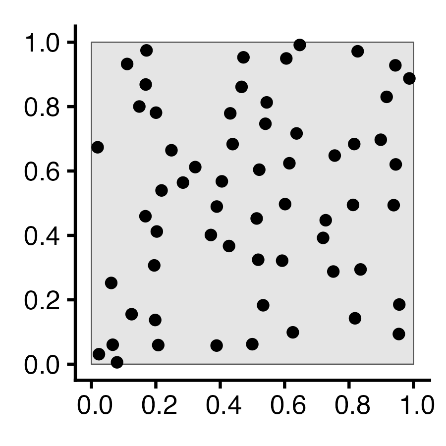
Original Data First-Order Second-Order
N = 60 Events Events modeled individually
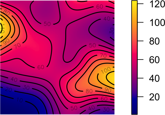
\Rightarrow Intensity Function \lambda(\mathbf{s})
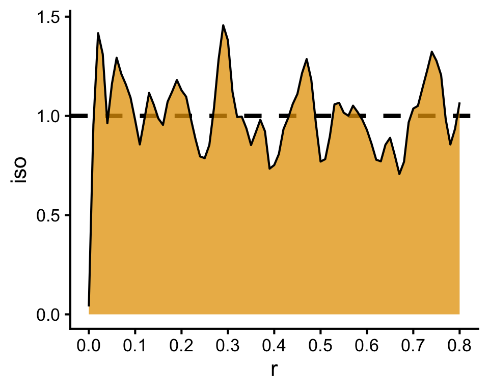
Events modeled pairwise \Rightarrow Pairwise-Corr Function \textrm{pcf}(\vec{h})

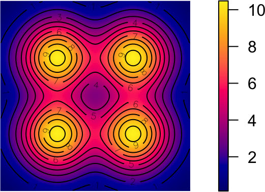
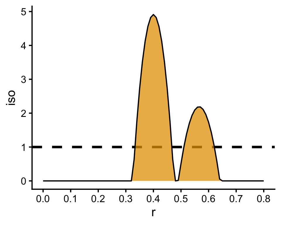
What Do These Functions “Detect”?

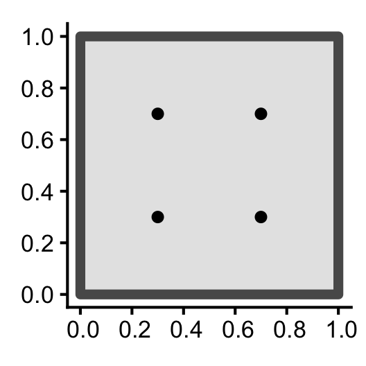
Code (Fixed Points)
sq_base <- 16
sq_psize <- 2.5
obs_window <- square(1)
r0 <- 0.2
sq_df <- tibble::tribble(
  ~x, ~y,
  0.5-r0,0.5-r0,
  0.5+r0,0.5+r0,
  0.5-r0,0.5+r0,
  0.5+r0,0.5-r0
)
sq_sf <- sf::st_as_sf(
  sq_df,
  coords = c("x","y")
)
sq_ppp <- as.ppp(sq_sf, W=obs_window)
sq_ppp |> sf::st_as_sf() |> ggplot() +
  geom_sf(size=sq_psize) +
  theme_classic(base_size=sq_base) +
  transparent_bg()

Code
par(
  mar=c(0,0,1,2),
  # mai=c(0,0,0.1,0),
  las=2,
  oma=c(0,0,1,0)
)
sq_density <- density(sq_ppp)
plot(sq_density, main=NULL, xaxs='i', yaxs='i', bg=NA)
contour(sq_density, xaxs='i', yaxs='i', add = TRUE)

Code
### PCF
pcf_result <- spatstat.explore::pcf(
  sq_ppp,
  divisor="d",
  r=seq(from=0.00, to=0.8, by=0.01)
)
pcf_result |> ggplot(aes(x=r, y=iso)) +
  geom_hline(yintercept=1, linetype='dashed', linewidth=1.5) +
  geom_area(color='black', fill=cb_palette[1], alpha=0.75) +
  scale_x_continuous(breaks=seq(from=0.0, to=1.0, by=0.1)) +
  theme_classic(base_size=sq_base) +
  transparent_bg()

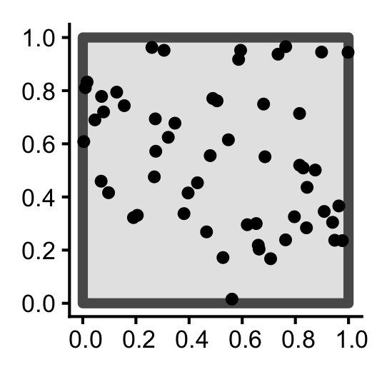
Code (CSR Points)
csr_ppp <- spatstat.random::rpoispp(
  lambda = 60,
  win=obs_window
)
csr_ppp |> sf::st_as_sf() |> ggplot() +
  geom_sf(size=sq_psize) +
  theme_classic(base_size=sq_base) +
  transparent_bg()

Code
par(
  mar=c(0,0,1,2),
  las=2,
  oma=c(0,0,1,0)
)
csr_density <- density(csr_ppp)
plot(csr_density, main=NULL, xaxs="i", yaxs="i", bg=NA)
contour(csr_density, xaxs="i", yaxs="i", add = TRUE, lwd=1.5)

Code
csr_pcf_result <- spatstat.explore::pcf(
  csr_ppp,
  divisor="d",
  r=seq(from=0.00, to=0.8, by=0.01)
)
csr_pcf_result |> ggplot(aes(x=r, y=iso)) +
  geom_hline(yintercept=1, linetype='dashed', linewidth=1.5) +
  geom_area(color='black', fill=cb_palette[1], alpha=0.75) +
  scale_x_continuous(breaks=seq(from=0.0, to=1.0, by=0.1)) +
  theme_classic(base_size=sq_base) +
  transparent_bg()

A Menagerie of Models

Open Interactive (WebR) Version

  • (…Interactivity is genuinely important here! Why? Hint:)

\begin{aligned} \text{Point Processes } \underbrace{\Omega}_{\mathclap{\text{Model of possible worlds}}} & ~~~~~~~~~~~~~\text{vs.} & \textit{Realizations}\text{ of Point Processes }\underbrace{\omega_1, \omega_2, \ldots}_{\mathclap{\text{Observed worlds}}} \end{aligned}

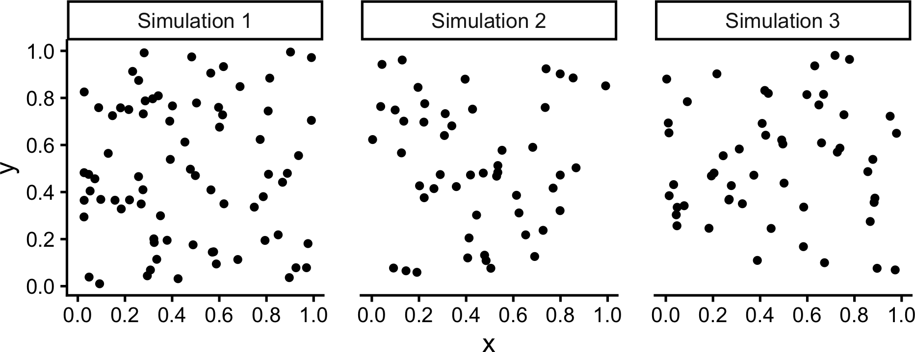
Poisson Point Processes (CSR)

spatstat.random::rpoispp(lambda, win)
  • N \sim \text{Pois}(\lambda)
  • For i \in \{1, \ldots, N\}:
    • Generate X_i, Y_i \sim \mathcal{U}(\texttt{win})
Code
sim_base <- 20
sim_psize <- 2
sim_xticks <- seq(from=0.0, to=1.0, by=0.2)
sim_yticks <- seq(from=0.0, to=1.0, by=0.2)
gen_pois_df <- function(num_sims=1) {
  pois_sims <- spatstat.random::rpoispp(
    lambda = 60, nsim=num_sims
  )
  return(tibble::as_tibble(pois_sims))
}
#pois_dfs <- gen_pois_df()
#pois_dfs |> head()
pois_sims <- spatstat.random::rpoispp(
  lambda = 60, nsim=3
)
to_sim_df <- function(cur_sim, sim_name) {
  cur_df <- tibble::as_tibble(cur_sim) |> mutate(sim=sim_name)
  return(cur_df)
}
combined_df <- imap(.x=pois_sims, .f=to_sim_df) |> bind_rows()
combined_df |> ggplot(aes(x=x, y=y)) +
  geom_point(size=sim_psize) +
  facet_wrap(vars(sim)) +
  coord_equal() +
  theme_classic(base_size=sim_base) +
  theme(panel.spacing.x = unit(2, "lines")) +
  scale_x_continuous(breaks=sim_xticks) +
  scale_y_continuous(breaks=sim_yticks) +
  transparent_bg()

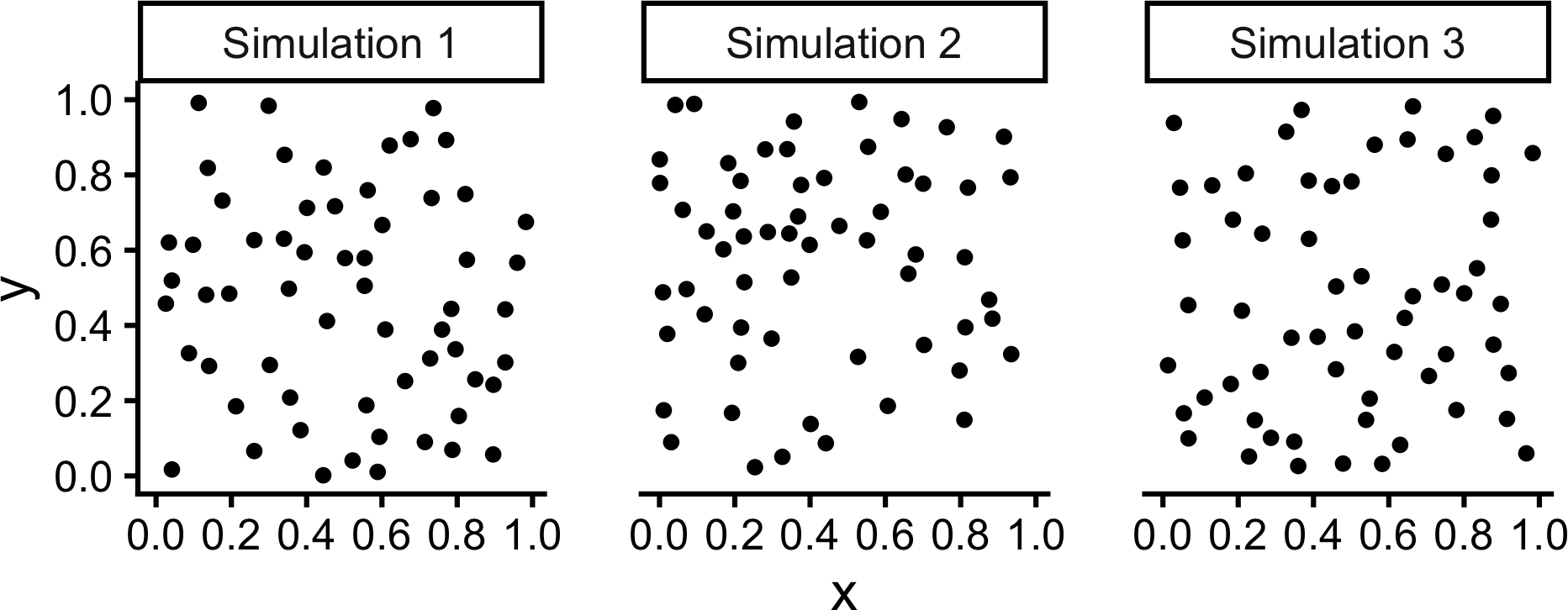
Simple Sequential Inhibition (SSI)

spatstat.random::rSSI(r, n=Inf, giveup=1000, win)
  • \mathbf{S} = \varnothing
  • While not done:
    • Generate \mathbf{E} = (X, Y) \sim \mathcal{U}(\texttt{win})
    • Check if \mathbf{E} within r units of any existing point in \mathbf{S}
      • If it is, throw \mathbf{E} away. Otherwise, add \mathbf{E} to \mathbf{S}
    • done=TRUE if \mathbf{S} has n points OR has been the same for giveup steps
Code
capture.output(ssi_sims <- spatstat.random::rSSI(
  r = 0.05, n=60, nsim=3
), file=nullfile())
combined_df <- imap(.x=ssi_sims, .f=to_sim_df) |> bind_rows()
combined_df |> ggplot(aes(x=x, y=y)) +
  geom_point(size=sim_psize) +
  facet_wrap(vars(sim)) +
  coord_equal() +
  theme_classic(base_size=24) +
  theme(panel.spacing.x = unit(3, "lines")) +
  scale_x_continuous(breaks=sim_xticks) +
  scale_y_continuous(breaks=sim_yticks) +
  transparent_bg()

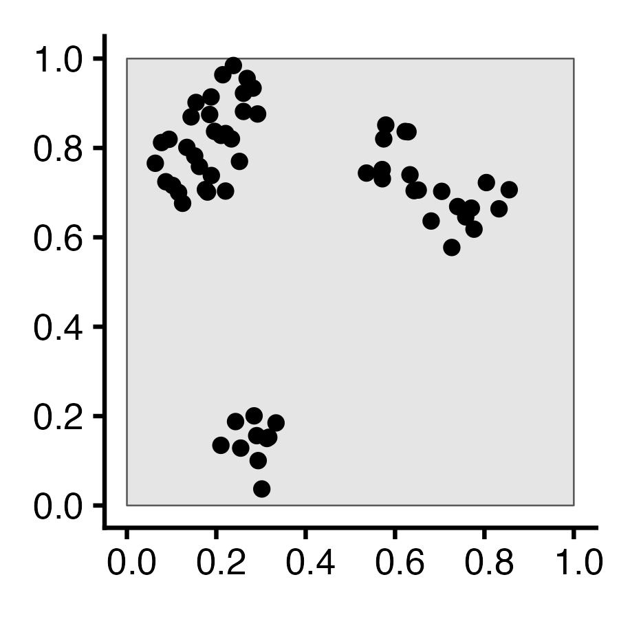
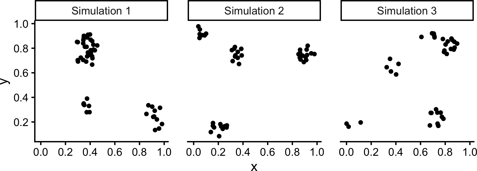
Matérn Cluster Process

spatstat.random::rMatClust(kappa, scale, mu, win)
  • Generate K(\kappa) parent points via Poisson Point Process with intensity \lambda = \kappa
  • For each parent point \mathbf{s}_i \in \left\{\mathbf{s}_1, \ldots, \mathbf{s}_{K(\kappa)}\right\}:
    • Generate N(\mu) offspring points via Poisson Point Process with intensity \lambda = \mu, distributed uniformly within a circle of radius scale centered at \mathbf{s}_i
  • Offspring points form the outcome (parent points are thrown away)
Code
matclust_sims <- rMatClust(
  kappa = 6,
  scale = 0.075,
  mu = 10,
  nsim = 3
)
matclust_df <- imap(.x=matclust_sims, .f=to_sim_df) |> bind_rows()
matclust_plot <- matclust_df |> ggplot(aes(x=x, y=y)) +
  geom_point(size=sim_psize) +
  facet_wrap(vars(sim), nrow=1) +
  coord_equal() +
  theme_classic(base_size=sim_base) +
  theme(panel.spacing.x = unit(2, "lines")) +
  scale_x_continuous(breaks=sim_xticks) +
  scale_y_continuous(breaks=sim_yticks) +
  transparent_bg()
matclust_plot

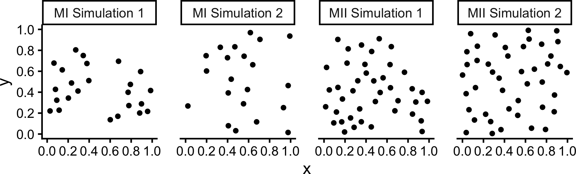
Matérn Inhibition Process (I and II)

spatstat.random::rMaternI(kappa, r, win)
spatstat.random::rMaternII(kappa, r, win)
rMaternI() [Docs] rMaternII() [Docs]
  • Generate events \mathbf{S} = \{\mathbf{s}_1, \ldots, \mathbf{s}_{N(\lambda)}\} via Poisson point process with \lambda = \kappa
  • Generate events \mathbf{S} = \{\mathbf{s}_1, \ldots, \mathbf{s}_{N(\lambda)}\} via Poisson point process with \lambda = \kappa, plus timestamp t_i \sim \mathcal{U}(0,1) for each \mathbf{s}_i
  • Delete all pairs of points \mathbf{s}_i, \mathbf{s}_j for which \textsf{dist}(\mathbf{s}_i, \mathbf{s}_j) < \texttt{r}
  • For each pair of points \mathbf{s}_i, \mathbf{s}_j: if \textsf{dist}(\mathbf{s}_i, \mathbf{s}_j) < \texttt{r}, delete the later point
Code
mI_sims <- rMaternI(
  kappa = 60, r = 0.075, nsim=2
)
mII_sims <- rMaternII(
  kappa = 60, r = 0.075, nsim=2
)
mI_combined_df <- imap(.x=mI_sims, .f=to_sim_df) |> bind_rows() |> mutate(sim=paste0("MI ",sim))
mII_combined_df <- imap(.x=mII_sims, .f=to_sim_df) |> bind_rows() |> mutate(sim=paste0("MII ",sim))
m_combined_df <- bind_rows(mI_combined_df, mII_combined_df)
m_plot <- m_combined_df |> ggplot(aes(x=x, y=y)) +
  geom_point(size=sim_psize) +
  facet_wrap(vars(sim), nrow=1) +
  coord_equal() +
  theme_classic(base_size=sim_base) +
  theme(panel.spacing.x = unit(2, "lines")) +
  scale_x_continuous(breaks=sim_xticks) +
  scale_y_continuous(breaks=sim_yticks) +
  transparent_bg()
m_plot

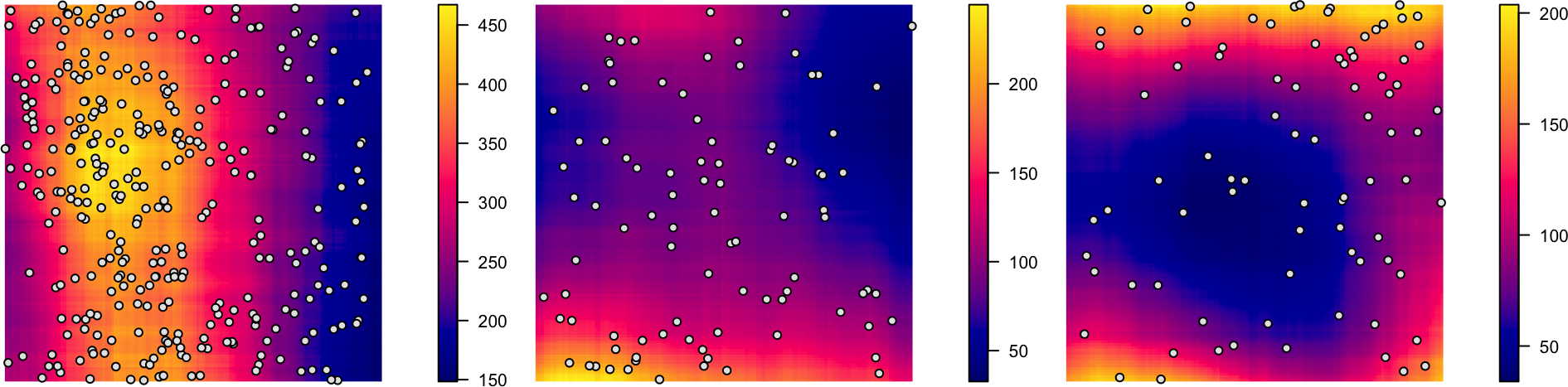
Cox Processes: Random Intensity → Random Events

spatstat.random::rLGCP(model, mu, param, win)
models=c("exponential", "gauss", "stable", "gencauchy", "matern")
Code
cox_pcol <- "black"
cox_bg <- "grey90"
cox_pch <- 21
# inhomogeneous LGCP with Gaussian covariance function
m <- as.im(function(x, y){
  5 - 1.5 * (x - 0.5)^2 + 2 * (y - 0.5)^2
}, W=owin())
lgcp_sims <- rLGCP("gauss", m, var=0.15, scale =0.5, nsim=3)
# lgcp_combined_df <- imap(.x=ssi_sims, .f=to_sim_df) |> bind_rows()
plot_lgcp <- function(lgcp_sim) {
  plot(attr(lgcp_sim, "Lambda"), main=NULL)
  points(lgcp_sim, col=cox_pcol, bg=cox_bg, pch=cox_pch)
}
par(mfrow=c(1,3), mar=c(0,0,0,2), oma=c(0,0,0,0), las=2)
nulls <- lapply(X=lgcp_sims, FUN=plot_lgcp)

Heterogeneous Point Processes

  • Cox Process highlights a crucial simplifying assumption we’ve made up til now: homogeneous point processes

    Homogeneous Point Process

    Points are distributed such that intensity \lambda, expected # of cases per unit area, is a constant across the study area

  • Allows “eyeballing” clusters: areas w/more points than expected under uniformity

  • But… in many cases we expect (e.g.) greater density of people in cities!

    Heterogeneous Point Process

    Distribution of points is determined by intensity function \lambda(\mathbf{s}), expected # of cases per unit area around \mathbf{s}

The Point: Base Rates \Rightarrow Null Models!

  • A “baseline” intensity function, \lambda(\mathbf{s}) (possibly c for all \mathbf{s}) defines a null model, from which we can simulate a bunch of point patterns…
  • Then we compare: How does an observed point pattern differ from these simulated point patterns?
  • Not expecting any clusters? Prior expectation = Uniform distribution \Rightarrow null model = homogeneous point process
    Do I see clustering? I \overset{\tiny{?}}{\gg} 0
  • Expecting clusters in cities? Prior expectation = Population density \Rightarrow null model = heterogeneous point process
    Do I see clustering above and beyond what I expected? I_{\text{obs}} \overset{\tiny{?}}{\gg} I_{\text{base}}

These Null Models Have Names!

  • Not expecting any clusters? Null model = Complete Spatial Randomness (CSR)
  • Expecting clusters (e.g.) in cities? Null model = Constant Risk Hypothesis
  • Why “constant risk”? From epidemiology:

\underbrace{\rho(\mathbf{s})}_{\text{Risk near }\mathbf{s}} ~~=~~~~~~ \frac{ \overbrace{\lambda(\mathbf{s})}^{\mathclap{\text{Density of cases near }s}} }{ \underbrace{\lambda_0(\mathbf{s})}_{\mathclap{\text{Population density near }\mathbf{s}}} }

Constant Risk Hypothesis: Motivation

  • Here is a (fictional) map of 2026 flu cases in the US “Midwest”
  • Are people in Chicago (pop. 2,731,585) and Detroit (pop. 649,095) equally “at risk”?
Code
library(mapview) |> suppressPackageStartupMessages()
city_df <- tibble::tribble(
  ~city, ~lon, ~lat, ~pop,
  "Chicago", 41.950567516553896, -87.93011127491978, 2746388,
  "Detroit", 42.45123004999075, -83.18402319217698, 631524
)
city_sf <- sf::st_as_sf(
  city_df,
  coords = c("lat", "lon"),
  crs=4326
)
city_buf_sf <- city_sf |> sf::st_buffer(20000)
city_cases_sf <- city_buf_sf |> sf::st_sample(size=rep(10,2)) |> sf::st_as_sf()
city_cases_sf$city <- "Detroit (10 Cases)"
city_cases_sf[1:10, 'city'] <- "Chicago (10 Cases)"
city_cases_sf$sample <- "Flu"
mapview(city_cases_sf, zcol="city")

Constant Risk Hypothesis: Base Rates

Chicago Detroit
Population 2,731,585 649,095
Code
library(leaflet) |> suppressPackageStartupMessages()
library(leaflet.extras2) |> suppressPackageStartupMessages()
city_pop_sf <- city_buf_sf |> sf::st_sample(size=c(16, 4)) |> sf::st_as_sf()
city_pop_sf$city <- "Detroit"
city_pop_sf[1:16, 'city'] <- "Chicago"
city_pop_sf$sample <- "People"
city_combined_sf <- bind_rows(city_cases_sf, city_pop_sf)
# mapview(city_combined_sf, zcol="city", marker="sample")
Flu = makeIcon(
    iconUrl="images/Maki2-danger-24.svg",
    iconRetinaUrl="images/Maki2-danger-24.svg",
    iconWidth=20,
    iconHeight=20,
    className='highlight-icon'
)
People = makeIcon(
  iconUrl="https://upload.wikimedia.org/wikipedia/commons/e/ef/Maki2-pitch-24.svg",
  iconRetinaUrl="https://upload.wikimedia.org/wikipedia/commons/e/ef/Maki2-pitch-24.svg",
  iconWidth=20,
  iconHeight=20,
  # className='boxed-cb'
)

city_combined_sf$r <- ifelse(city_combined_sf$sample == "Flu", 0, 4)
city_flu_sf <- city_combined_sf |> filter(sample == "Flu")
city_ppl_sf <- city_combined_sf |> filter(sample == "People")
leaflet(city_flu_sf) |>
  addProviderTiles("Esri.WorldGrayCanvas") |>
  # addProviderTiles("CartoDB.Positron") |>
  addMarkers(data=city_flu_sf, icon = Flu) |>
  addMarkers(data=city_ppl_sf, icon = People)

Example from Moraga (2024)

Code
library(sparr) |> suppressPackageStartupMessages()
data(pbc)
controls <- unmark(pbc[which(pbc$marks == "control"), ])
controls |> sf::st_as_sf() |> ggplot() +
  geom_sf() +
  theme_classic() +
  labs(title="Controls (Population Sample)") +
  transparent_bg()

Code
cases <- unmark(pbc[which(pbc$marks == "case"), ])
cases |> sf::st_as_sf() |> ggplot() +
  geom_sf() +
  theme_classic() +
  labs(title="PBC Cases") +
  transparent_bg()

Estimating Comparable Intensity Surfaces

  • To ensure comparable intensity functions, need a common bandwidth value
  • density() from spatstat makes “smart” choices for this bandwidth, so for now we just average the bandwidths estimated for cases and controls:
Code
library(sparr)
data(pbc)
par(mar=c(2,0,2,0))
cases <- unmark(pbc[which(pbc$marks == "case"), ])
controls <- unmark(pbc[which(pbc$marks == "control"), ])
bwcases <- attr(density(cases), "sigma")
bwcontr <- attr(density(controls), "sigma")
(bw <- (bwcases + bwcontr)/2)
[1] 11.45837
Code
int_controls <- density(controls, sigma = bw, eps=0.25)
plot(int_controls, main = "λ(Controls)", bg=NA)

Code
int_cases <- density(cases, sigma = bw, eps=0.25)
plot(int_cases, main = "λ(Cases)", bg=NA)

Visualizing Relative Risk Surface

To account for N_0 \neq N, normalize numerator and denominator:

\hat{\rho}(\mathbf{s}) = \frac{\hat{\lambda}(\mathbf{s}) / N}{\hat{\lambda}_0(\mathbf{s}) / N_0}

\Rightarrow \hat{\rho}(\mathbf{s}) = \frac{\hat{\lambda}(\mathbf{s})}{\alpha\hat{\lambda}_0(\mathbf{s})}, where \alpha = \frac{N}{N_0}

Code
(alpha <- cases$n/controls$n)
[1] 0.2519868
Code
library(fields)
library(scico)
x <- int_cases$xcol
y <- int_cases$yrow
rr <- t(int_cases$v)/t(alpha * int_controls$v)
center <- 1.0
lim <- max(abs(rr - center), na.rm = TRUE)
# pal <- colorRampPalette(c("#2166AC", "white", "#B2182B"))(101)
par(
  mar=c(6.5,3,1.5,0.5),
  oma=c(1,1,1,1),
  xpd=NA,
  mgp = c(1.6, 0.6, 0)
)
pal <- scico(101, palette = "vik")
image.plot(x, y, rr, asp = 1, col=pal, zlim = c(center - lim, center + lim), main="Relative Risk Surface", xlab="Easting", ylab="Northing", bty='l')

From Exploratory to Confirmatory Data Analysis

  • How do we know whether ↑ risk around North Newcastle due to “chance”? Maybe relative risk is actually constant, and people in Newcastle are just unlucky…
  • Thought experiment: Bro hands you a coin. You flip 10 times. HHHHHTHHHH…
  • Coin may be biased-towards-H, or could be fair (lots of heads by chance!)
  • Stats: Compare with null model! For fair coin, how likely is [9 Heads / 10 Flips]?

Exploratory Data Analysis: Collecting evidence

Confirmatory Data Analysis: Making judgements

Null Model: CSR

Figure from Gimond (2024)

The Random Labeling Hypothesis

  • Randomly apply 761 “sick” labels to the 761 + 3020 = 3781 points!
Code
plot_rlabel <- function(rl_ppp) {
  rl_win_sf <- window_to_sf(rl_ppp)
  rl_points_sf <- points_to_sf(rl_ppp) |>
    rename(
      type = spatstat.geom..marks.x.
    )
  rl_plot <- ggplot() +
    geom_sf(
      data=rl_win_sf,
      alpha=0.3
    ) +
    geom_sf(
      mapping=aes(fill=type, alpha=type),
      data=rl_points_sf,
      size=2,
      # alpha=0.75,
      shape=21,
      stroke=0.1,
      # color='white',
    ) +
    # scale_color_manual(
    #   "Point Type",
    #   values=c("control"="gray","case"=cb_palette[1])
    # ) +
    scale_fill_manual(
      "Type",
      values=c("control"="gray","case"=cb_palette[1])
    ) +
    scale_alpha_manual(
      "Type",
      values=c("control"=0.5, "case"=1.0)
    ) +
    theme_classic(base_size=16) +
    labs(
      title="NE Britain Disease Cases"
    ) +
    transparent_bg()
  return(rl_plot)
}
set.seed(6810)
rl1_ppp <- rlabel(pbc)
plot_rlabel(rl1_ppp)

Code
set.seed(6811)
pbc_2 <- rlabel(pbc)
plot_rlabel(pbc_2)

Code
set.seed(6812)
pbc_3 <- rlabel(pbc)
plot_rlabel(pbc_3)

The Constant Risk Hypothesis

  • Everyone equally at risk of contracting disease, regardless of location: \rho(\mathbf{s}) = 1
  • In this case: \lambda_{CR}(\mathbf{s}) = \alpha \lambda_0(\mathbf{s}) (some constant \alpha \times base rate \lambda_0(\mathbf{s}))
Code
pbc_win_sf <- pbc |> sf::st_as_sf() |> filter(label == "window")
plot_pbc_sim <- function() {
    pbc_sim <- spatstat.random::rpoispp(
        lambda = alpha * int_controls
    )
    # Separate window and points
    pbc_sf <- pbc_sim |> sf::st_as_sf()
    pbc_point_sf <- pbc_sf |> filter(label == "point")
    pbc_win_sf <- pbc_sf |> filter(label == "window")
    pbc_plot <- ggplot() +
      geom_sf(data=pbc_win_sf) +
      geom_sf(data=pbc_point_sf, size=0.5, alpha=0.5) +
      theme_classic() +
      transparent_bg()
    return(pbc_plot)
}
plot_pbc_sim()

Code
plot_pbc_sim()

Code
plot_pbc_sim()

HW3 Tips!

  • ppp Objects
  • Converting between ppp and sf
  • Plotting

ppp Objects

  • The main datatype used to represent Planar Point Patterns [spatstat book p. 41]
  • Unlike sf objects, which contain data+geometries for any desired collection of N entities, ppp objects are required to have at least an observation window!

sf Creation:

Code
tree_df <- tibble::tibble(
  lon=runif(100,0,1), lat=runif(100,0,1), age=runif(100,0,1)
)
tree_sf <- sf::st_as_sf(
  tree_df, coords = c('lon', 'lat')
)
tree_sf |> head(4)
age geometry
0.4083865 POINT (0.9493056 0.7413338)
0.2109350 POINT (0.4885575 0.626284)
0.1177755 POINT (0.1203148 0.2863668)
0.7475464 POINT (0.6020442 0.4303325)

ppp Creation:

Code
pois_ppp <- spatstat.random::rpoispp(
  lambda=100, win=spatstat.geom::square(1)
)
pois_ppp
Planar point pattern: 98 points
window: rectangle = [0, 1] x [0, 1] units
Code
attributes(pois_ppp)$names
[1] "window"     "n"          "x"          "y"          "markformat"
Code
pois_ppp$x |> head(4)
[1] 0.7185641 0.9781310 0.1744719 0.4256203

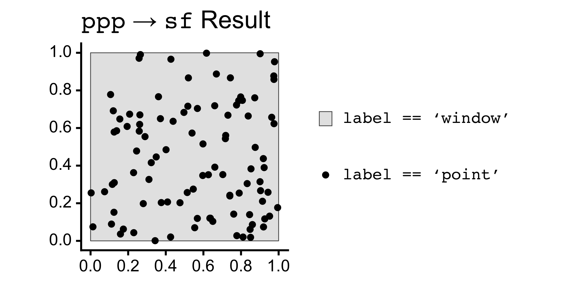
ppp \leftrightarrow sf Conversion

ppp to sf Conversion:

Code
pois_sf <- pois_ppp |> sf::st_as_sf()
pois_sf |> head(4)
label geom
window POLYGON ((0 0, 1 0, 1 1, 0 …
point POINT (0.7185641 0.5606081)
point POINT (0.978131 0.9523815)
point POINT (0.1744719 0.06257196)
Code
library(mdthemes) |> suppressPackageStartupMessages()
pois_sf |> ggplot() +
  geom_sf(data=pois_sf |> filter(label=="window"), aes(fill='grey')) +
  geom_sf(data=pois_sf |> filter(label != "window"), aes(color='black')) +
  md_theme_classic(base_size=26) +
  scale_fill_manual(name=NULL, values=c("gray90"), labels=c("<span style='font-family: mono'>label == 'window'</span>")) +
  scale_color_manual(name=NULL, values=c("black"), labels=c("<span style='font-family: mono'>label == 'point'</span>")) +
  labs(title = "<span style='font-family: mono'>ppp</span> &rarr; <span style='font-family: mono'>sf</span> Result") +
  transparent_bg()

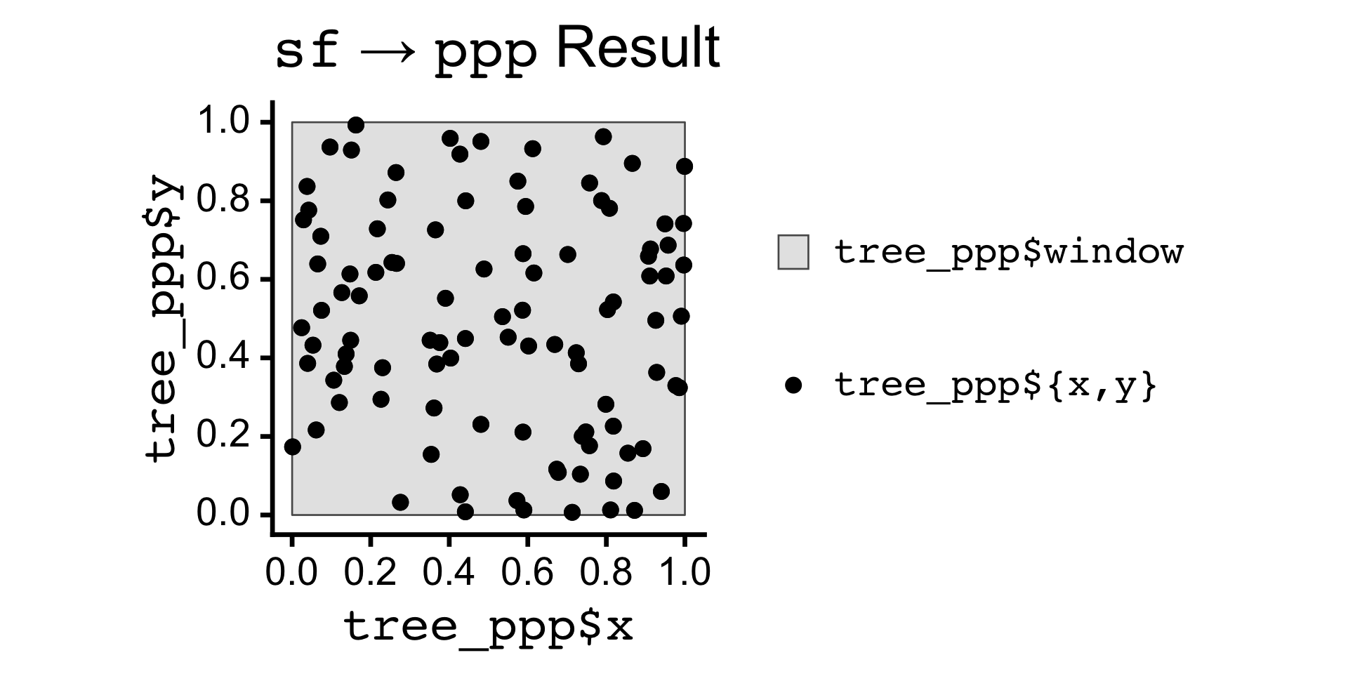
sf to ppp Conversion:

Code
square_sfc <- sf::st_polygon(list(
  matrix(c(0,0,1,0,1,1,0,1,0,0), nrow=5, byrow=TRUE)
)) |> sf::st_sfc()
tree_ppp <- as.ppp(
  sf::st_as_sfc(tree_sf),
  W=as.owin(square_sfc)
)
tree_ppp
Planar point pattern: 100 points
window: polygonal boundary
enclosing rectangle: [0, 1] x [0, 1] units
Code
tree_ppp_sf <- tree_ppp |> sf::st_as_sf()
tree_ppp_sf |> ggplot() +
  geom_sf(aes(fill='gray90')) +
  geom_sf(data=tree_ppp_sf |> filter(label != "window"), aes(color='black')) +
  md_theme_classic(base_size=26) +
  scale_fill_manual(name=NULL, values=c("gray90"), labels=c("<span style='font-family: mono'>tree_ppp$window</span>")) +
  scale_color_manual(name=NULL, values=c("black"), labels=c("<span style='font-family: mono'>tree_ppp${x,y}</span>")) +
  labs(
    title = "<span style='font-family: mono'>sf</span> &rarr; <span style='font-family: mono'>ppp</span> Result",
    x="<span style='font-family: mono'>tree_ppp$x</span>",
    y="<span style='font-family: mono'>tree_ppp$y</span>"
  ) + 
  guides(
    fill = guide_legend(order = 1),
    color = guide_legend(order = 2)
  ) +
  transparent_bg()

References

Gimond, Manuel. 2024. Introduction to GIS and Spatial Analysis. Colby College (ES214).