Week 11: Double-Checking Is Possible, Infinity-Checking Is Not (Robustness and Sensitivity Analysis)

DSAN 5650: Causal Inference for Computational Social Science
Summer 2026, Georgetown University

Jeff Jacobs

jj1088@georgetown.edu

Wednesday, July 29, 2026

Final Project Progress Report / Draft: Friday, 11:59pm EDT

Robustness and Sensitivity Analysis: Complementary!

Car Safety Metaphor

  • Robustness: Doing stuff to maximize “safety” (from getting causal effect wrong)
Seatbelts Installed?Covariates Adjusted?
No Yes
Airbag Installed?Propensity Score Estimated? No OLS OLS + "Controls"
Yes IPW Doubly Robust! 🥳
  • Sensitivity Analysis: What is the “breaking point” of my safety measures?
  • \(\Pr(\)Not enough time for airbag to inflate\() \propto\) speed
  • \(\leadsto\) Over 100mph, \(\Pr(\)Not enough time for airbag to inflate\() > 0.95\)
  • \(\Pr(\)Wrong causal effect\() \propto\) correlation of omitted confounder with treatment, outcome
  • \(\leadsto\) Over \(\rho = 0.6\), \(\Pr(\)Wrong causal effect\() > 0.95\)

Sensitivity Analysis 2: How Sensitive Are My Results to Included Variable Bias?

  • You probably know about omitted variable bias from previous classes / intuition… but, included variable bias?
  • That’s right folks… colliders can be agents of chaos, laying waste to our best, most meticulously-planned-out models

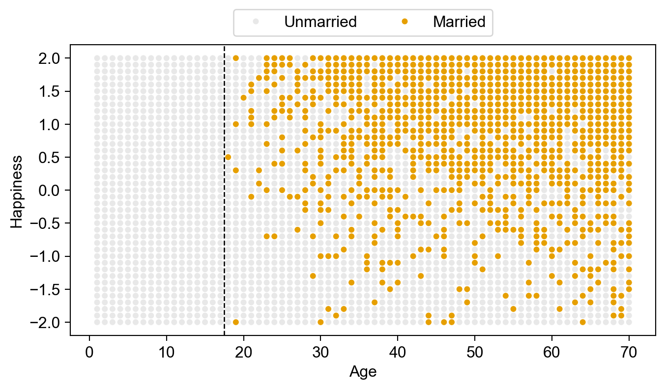
Does Aging Cause Sadness?

Each year, 20 people are born with uniformly-distributed happiness values
Each year, each person ages one year; Happiness does not change
At age 18, individuals can become married; Odds of marriage each year proportional to individual's happiness; Once married, they remain married
At age 70 individuals leave the sample (They move to Boca Raton, Florida)
Code
import pandas as pd
import numpy as np
rng = np.random.default_rng(seed=5650)
import matplotlib.pyplot as plt
import seaborn as sns
cb_palette = ['#e69f00','#56b4e9','#009e73']
sns.set_palette(cb_palette)
from scipy.special import expit

# The original R code:
# sim_happiness <- function( seed=1977 , N_years=1000 , max_age=65 , N_births=20 , aom=18 ) {
#     set.seed(seed)
#     H <- M <- A <- c()
#     for ( t in 1:N_years ) {
#         A <- A + 1 # age existing individuals
#         A <- c( A , rep(1,N_births) ) # newborns
#         H <- c( H , seq(from=-2,to=2,length.out=N_births) ) # sim happiness trait - never changes
#         M <- c( M , rep(0,N_births) ) # not yet married
#         # for each person over 17, chance get married
#         for ( i in 1:length(A) ) {
#             if ( A[i] >= aom & M[i]==0 ) {
#                 M[i] <- rbern(1,inv_logit(H[i]-4))
#             }
#         }
#         # mortality
#         deaths <- which( A > max_age )
#         if ( length(deaths)>0 ) {
#             A <- A[ -deaths ]
#             H <- H[ -deaths ]
#             M <- M[ -deaths ]
#        }
#     }
#     d <- data.frame(age=A,married=M,happiness=H)
#     return(d)

# DGP: happiness -> marriage <- age
years = 70
num_births = 41
colnames = ['age','a','h','m']
sim_dfs = []
A = np.zeros(shape=(num_births,1))
H = np.linspace(-2, 2, num=num_births)
M = np.zeros(shape=(num_births,1))
def update_m(row):
  if row['m'] == 0:
    return int(rng.binomial(
      n=1,
      p=expit(row['h'] - 3.875),
      size=1,
    )[0])
  return 1
def sim_cohort_to(max_age):
  sim_df = pd.DataFrame({
      'age': [1 for _ in range(num_births)],
      'h': np.linspace(-2, 2, num=num_births),
      'm': [0 for _ in range(num_births)],
    }
  )
  for t in range(2, max_age + 1):
    sim_df['age'] = sim_df['age'] + 1
    if t >= 18:
      sim_df['m'] = sim_df.apply(update_m, axis=1)
  return sim_df
all_sim_dfs = []
for cur_max_age in range(1, 71):
  cur_sim_df = sim_cohort_to(cur_max_age)
  all_sim_dfs.append(cur_sim_df)
full_sim_df = pd.concat(all_sim_dfs)

# And plot
fig, ax = plt.subplots(figsize=(8, 4))
cbg_palette = ['#c6c6c666'] + cb_palette
full_sim_df['m_label'] = full_sim_df['m'].apply(lambda x: "Unmarried" if x == 0 else "Married")
full_sim_df = full_sim_df.rename(columns={'age': 'Age', 'h': 'Happiness'})
happiness_plot = sns.scatterplot(
  x='Age', y='Happiness', hue='m_label',
  data=full_sim_df,
  palette=cbg_palette[:2],
  s=24,
  ax=ax,
  legend=True,
);
# happiness_plot.move_legend("upper center", bbox_to_anchor=(0.5, 1.15), ncol=2);
sns.move_legend(ax, "upper center", bbox_to_anchor=(0.5, 1.15), ncol=2);
happiness_plot.legend_.set_title("");
happiness_plot.axvline(x=17.5, color='black', ls='dashed', lw=1);
plt.show();

Happiness by Age, 70 birth cohorts of size 41 each (DC minimum marriage age = 18)

…What’s happening here?
\(\textsf{Happy} \rightarrow {}^{🤔}\textsf{Marriage}^{🤔} \leftarrow \textsf{Age}\)

Sensitivity Analysis 3: How Sensitive Are My Results to Omitted Variable Bias?

Assessing the Impact of Omitted Vars

  • Working example: PCPSR, People’s Company for Public Survey Research (شركة الشعب الأبحاث المسحية)
  • What is causal impact of experiencing violence on support for armed struggle?
  • Researcher A models this scenario as:

\[ \textsf{ArmedStruggle}_i = \alpha^\text{res} + \tau^\text{res} \textsf{DirectHarm}_i + \hat{\beta}_\text{c}^\text{res}\textsf{RefugeeCamp}_i + \textsf{Muhaf}_i \hat{\boldsymbol \beta}_\text{m}^\text{res} + \hat{\varepsilon}^\text{res} \]

  • Researcher B instead prefers:

\[ \textsf{ArmedStruggle}_i = \alpha + \tau \textsf{DirectHarm}_i + \hat{\beta}_\text{c}\textsf{RefugeeCamp}_i + \textsf{Muhaf}_i \hat{\boldsymbol \beta}_{\text{m}} + \boxed{\hat{\gamma}\textsf{PFLP}_i} + \hat{\varepsilon}^{\text{full}} \]

Our earlier estimate \(\tau_{\text{res}}\) would differ from our target quantity \(\tau\): but how badly?

How strong would the confounder(s) have to be to change the estimates in such a way to affect the main conclusions of a study?

The Classical OVB Equation

  • Remember that \(T\) is our treatment variable! (\(\mathbf{X}\) = covariates, \(Y\) = outcome)
  • In a perfect world, we would estimate \(Y = \hat{\tau}T + \mathbf{X} \hat{\beta} + \hat{\gamma}Z+ \varepsilon_{\text{full}}\)
  • But, \(Z\) is unobserved \(\leadsto\) “restricted” model \(Y = \hat{\tau}_{\text{res}}T + \mathbf{X} \hat{\beta}_{\text{res}} + \varepsilon_{\text{res}}\)
  • What is the “gap” between \(\hat{\tau}\) and \(\hat{\tau}^{\text{res}}\)? \(\text{OVB} = \hat{\tau}_{\text{res}} - \hat{\tau}\)

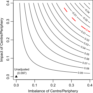
\[ \begin{align*} \hat{\tau}_{\text{res}} &= \frac{ \text{Cov}[T^{\top \mathbf{X}}, Y^{\top \mathbf{X}}] }{ \text{Var}[T^{\top \mathbf{X}}] } \\ &= \frac{ \text{Cov}[T^{\top \mathbf{X}}, \hat{\tau}T^{\top \mathbf{X}} + \hat{\gamma}Z^{\top \mathbf{X}}] }{ \text{Var}[T^{\top \mathbf{X}}] } \\ &= \hat{\tau} + \hat{\gamma}\frac{ \text{Cov}[T^{\top \mathbf{X}}, Z^{\top \mathbf{X}}] }{ \text{Var}[T^{\top \mathbf{X}}] } \\ &= \hat{\tau} + \hat{\gamma}\hat{\delta} \\ \implies \text{OVB} &= \hat{\tau}_{\text{res}} - \hat{\tau} = \overbrace{ \boxed{\hat{\gamma} \times \hat{\delta}} }^{\mathclap{\text{Impact} \, \times \, \text{Imbalance}}} \end{align*} \]
More Generally

  • What if we don’t have a specific omitted variable in mind? We just want to know the expected impact if there were omitted vars… Enter “Partial \(R^2\)

References